Python High Performance
Programming
Boost the performance of your Python programs
using advanced techniques
Gabriele Lanaro
BIRMINGHAM - MUMBAI
Python High Performance Programming
Copyright © 2013 Packt Publishing
All rights reserved. No part of this book may be reproduced, stored in a retrieval system, or transmitted in any form or by any means, without the prior written permission of the publisher, except in the case of brief quotations embedded in critical articles or reviews.
Every effort has been made in the preparation of this book to ensure the accuracy of the information presented. However, the information contained in this book is sold without warranty, either express or implied. Neither the author, nor Packt Publishing, and its dealers and distributors will be held liable for any damages caused or alleged to be caused directly or indirectly by this book.
Packt Publishing has endeavored to provide trademark information about all of the companies and products mentioned in this book by the appropriate use of capitals. However, Packt Publishing cannot guarantee the accuracy of this information.
First published: December 2013
Production Reference: 1171213
Published by Packt Publishing Ltd. Livery Place
35 Livery Street
Birmingham B3 2PB, UK.
ISBN 978-1-78328-845-8
www.packtpub.com
Credits
Author
Gabriele Lanaro
Reviewers Daniel Arbuckle
Mike Driscoll
Albert Lukaszewski
Acquisition Editors Owen Roberts
Harsha Bharwani
Commissioning Editor Shaon Basu
Technical Editors Akashdeep Kundu
Faisal Siddiqui
Project Coordinator Sherin Padayatty
Proofreader Linda Morris
Indexer Rekha Nair
Production Coordinators Pooja Chiplunkar
Manu Joseph
Cover Work Pooja Chiplunkar
About the Author
Gabriele Lanaro
is a PhD student in Chemistry at the University of British Columbia, in the field of Molecular Simulation. He writes high performance Python code to analyze chemical systems in large-scale simulations. He is the creator of Chemlab—a high performance visualization software in Python—and emacs-for-python—a collection of emacs extensions that facilitate working with Python code in the emacs text editor. This book builds on his experience in writing scientific Python code for his research and personal projects.I want to thank my parents for their huge, unconditional love and support. My gratitude cannot be expressed by words but I hope that I made them proud of me with this project.
I would also thank the Python community for producing and maintaining a massive quantity of high-quality resources made available for free. Their extraordinary supportive and compassionate attitude really fed my passion for this amazing technology.
About the Reviewers
Dr. Daniel Arbuckle is a published researcher in the fields of robotics and
nanotechnology, as well as a professional Python programmer. He is the author of Python Testing: Beginner's Guide from Packt Publishing and one of the authors of Morphogenetic Engineering from Springer-Verlag.Mike Driscoll has been programming in Python since Spring 2006. He enjoys
writing about Python on his blog at http://www.blog.pythonlibrary.org/. Mike also occasionally writes for the Python Software Foundation, i-Programmer, and Developer Zone. He enjoys photography and reading a good book. Mike has also been a technical reviewer for Python 3 Object Oriented Programming, Python 2.6 Graphics Cookbook, and Tkinter GUI Application Development Hotshot.I would like to thank my beautiful wife, Evangeline, for always supporting me. I would also like to thank friends and family for all that they do to help me. And I would like to thank Jesus Christ for saving me.
Albert Lukaszewski
is a software consultant and the author of MySQL for Python. He has programmed computers for nearly 30 years. He specializes in high-performance Python implementations of network and database services. He has designed and developed Python solutions for a wide array of industries including media, mobile, publishing, and cinema. He lives with his family in southeast Scotland.www.PacktPub.com
Support files, eBooks, discount offers and more
You might want to visit www.PacktPub.com for support files and downloads related to your book.
Did you know that Packt offers eBook versions of every book published, with PDF and ePub files available? You can upgrade to the eBook version at www.PacktPub. com and as a print book customer, you are entitled to a discount on the eBook copy. Get in touch with us at [email protected] for more details.
At www.PacktPub.com, you can also read a collection of free technical articles, sign up for a range of free newsletters and receive exclusive discounts and offers on Packt books and eBooks.
TM
http://PacktLib.PacktPub.com
Do you need instant solutions to your IT questions? PacktLib is Packt's online digital book library. Here, you can access, read and search across Packt's entire library of books.
Why Subscribe?
• Fully searchable across every book published by Packt • Copy and paste, print and bookmark content
• On demand and accessible via web browser
Free Access for Packt account holders
Table of Contents
Preface 1
Chapter 1: Benchmarking and Profiling
7
Designing your application 7
Writing tests and benchmarks 13
Timing your benchmark 15
Finding bottlenecks with cProfile 17 Profile line by line with line_profiler 21
Optimizing our code 23
The dis module 25
Profiling memory usage with memory_profiler 26 Performance tuning tips for pure Python code 28
Summary 30
Chapter 2: Fast Array Operations with NumPy
31
Getting started with NumPy 31
Creating arrays 32
Accessing arrays 34
Broadcasting 37
Mathematical operations 40
Calculating the Norm 41
Rewriting the particle simulator in NumPy 41 Reaching optimal performance with numexpr 45
Summary 47
[ ii ]
Chapter 3: C Performance with Cython
49
Compiling Cython extensions 49
Adding static types 52
Variables 52 Functions 54 Classes 55
Sharing declarations 56
Working with arrays 58
C arrays and pointers 58
NumPy arrays 60
Typed memoryviews 61
Particle simulator in Cython 63
Profiling Cython 67
Summary 70
Chapter 4: Parallel Processing
71
Introduction to parallel programming 72 The multiprocessing module 74
The Process and Pool classes 74
Monte Carlo approximation of pi 77
Synchronization and locks 80
IPython parallel 82
Direct interface 83
Task-based interface 87
Parallel Cython with OpenMP 88
Summary 91
Preface
Python is a programming language renowned for its simplicity, elegance, and the support of an outstanding community. Thanks to the impressive amount of high-quality third-party libraries, Python is used in many domains.
Low-level languages such as C, C++, and Fortran are usually preferred in performance-critical applications. Programs written in those languages perform extremely well, but are hard to write and maintain.
Python is an easier language to deal with and it can be used to quickly write complex applications. Thanks to its tight integration with C, Python is able to avoid the performance drop associated with dynamic languages. You can use blazing fast C extensions for performance-critical code and retain all the convenience of Python for the rest of your application.
In this book, you will learn, in a step-by-step method how to find and speedup the slow parts of your programs using basic and advanced techniques.
The style of the book is practical; every concept is explained and illustrated with examples. This book also addresses common mistakes and teaches how to avoid them. The tools used in this book are quite popular and battle-tested; you can be sure that they will stay relevant and well-supported in the future.
This book starts from the basics and builds on them, therefore, I suggest you to move through the chapters in order.
And don't forget to have fun!
What this book covers
Chapter 1, Benchmarking and Profiling shows you how to find the parts of your program that need optimization. We will use tools for different use cases and explain how to analyze and interpret profiling statistics.
Chapter 2, Fast Array Operations with NumPy is a guide to the NumPy package. NumPy is a framework for array calculations in Python. It comes with a clean and concise API, and efficient array operations.
Chapter3, C Performance with Cython is a tutorial on Cython: a language that acts as a bridge between Python and C. Cython can be used to write code using a superset of the Python syntax and to compile it to obtain efficient C extensions.
Chapter4, Parallel Processing is an introduction to parallel programming. In this chapter, you will learn how parallel programming is different from serial programming and how to parallelize simple problems. We will also explain how to use multiprocessing, IPython.parallel and cython.parallel to write code for multiple cores.
What you need for this book
This book requires a Python installation. The examples work for both Python 2.7 and Python 3.3 unless indicated otherwise.
In this book, we will make use of some popular Python packages:
• NumPy (Version 1.7.1 or later): This package is downloadable from the official website (http://www.scipy.org/scipylib/download.html) and available in most of the Linux distributions
• Cython (Version 0.19.1 or later): Installation instructions are present in the official website (http://docs.cython.org/src/quickstart/install. html); notice that you also need a C compiler, such as GCC (GNU Compiler Collection), to compile your C extensions
• IPython (Version 0.13.2 or later): Installation instructions are present in the official website (http://ipython.org/install.html)
The book was written and tested on Ubuntu 13.10. The examples will likely run on Mac OS X with little or no changes.
[ 3 ]
A convenient alternative is to use the free service wakari.io: a cloud-based Linux and Python environment that includes the required packages with their tools and utilities. No setup is required.
In Chapter 1, Benchmarking and Profiling, we will use KCachegrind (http:// sourceforge.net/projects/kcachegrind/), which is available for Linux.
KCachegrind has also a port for Windows—QcacheGrind—which is also installable from source on Mac OS X.
Who this book is for
This book is for intermediate to advanced Python programmers who develop performance-critical applications. As most of the examples are taken from scientific applications, the book is a perfect match for scientists and engineers looking to speed up their numerical codes.
However, the scope of this book is broad and the concepts can be applied to any domain. Since the book addresses both basic and advanced topics, it contains useful information for programmers with different Python proficiency levels.
Conventions
In this book, you will find a number of styles of text that distinguish between different kinds of information. Here are some examples of these styles, and an explanation of their meaning.
Code words in text, database table names, folder names, filenames, file extensions, pathnames, dummy URLs, user input, and Twitter handles are shown as follows: "The plot function included in matplotlib can display our particles as points on a Cartesian grid and the FuncAnimation class can animate the evolution of our particles over time."
A block of code is set as follows:
from matplotlib import pyplot as plt from matplotlib import animation
def visualize(simulator):
When we wish to draw your attention to a particular part of a code block, the relevant lines or items are set in bold:
In [1]: import purepy
In [2]: %timeit purepy.loop()
100 loops, best of 3: 8.26 ms per loop In [3]: %timeit purepy.comprehension() 100 loops, best of 3: 5.39 ms per loop In [4]: %timeit purepy.generator() 100 loops, best of 3: 5.07 ms per loop
Any command-line input or output is written as follows:
$ time python simul.py # Performance Tuned
real 0m0.756s
user 0m0.714s
sys 0m0.036s
New terms and important words are shown in bold. Words that you see on the screen, in menus or dialog boxes, for example, appear in the text like this: "You can navigate to the Call Graph or the Caller Map tabs by double-clicking on the rectangles."
Warnings or important notes appear in a box like this.
Tips and tricks appear like this.
Reader feedback
Feedback from our readers is always welcome. Let us know what you think about this book—what you liked or may have disliked. Reader feedback is important for us to develop titles that you really get the most out of.
To send us general feedback, simply send an e-mail to [email protected], and mention the book title via the subject of your message.
[ 5 ]
Customer support
Now that you are the proud owner of a Packt book, we have a number of things to help you to get the most from your purchase.
Downloading the example code
You can download the example code files for all Packt books you have purchased from your account at http://www.packtpub.com. If you purchased this book elsewhere, you can visit http://www.packtpub.com/support and register to have the files e-mailed directly to you.
Errata
Although we have taken every care to ensure the accuracy of our content, mistakes do happen. If you find a mistake in one of our books—maybe a mistake in the text or the code—we would be grateful if you would report this to us. By doing so, you can save other readers from frustration and help us improve subsequent versions of this book. If you find any errata, please report them by visiting http://www.packtpub. com/submit-errata, selecting your book, clicking on the erratasubmissionform link, and entering the details of your errata. Once your errata are verified, your submission will be accepted and the errata will be uploaded on our website, or added to any list of existing errata, under the Errata section of that title. Any existing errata can be viewed by selecting your title from http://www.packtpub.com/support.
Piracy
Piracy of copyright material on the Internet is an ongoing problem across all media. At Packt, we take the protection of our copyright and licenses very seriously. If you come across any illegal copies of our works, in any form, on the Internet, please provide us with the location address or website name immediately so that we can pursue a remedy.
Please contact us at [email protected] with a link to the suspected pirated material.
We appreciate your help in protecting our authors, and our ability to bring you valuable content.
Questions
Benchmarking and Profiling
Recognizing the slow parts of your program is the single most important task when it comes to speeding up your code. In most cases, the bottlenecks account for a very small fraction of the program. By specifically addressing those critical spots you can focus on the parts that needimprovement without wasting time in micro-optimizations.
Profiling is the technique that allows us to pinpoint the bottlenecks. A profiler is a program that runs the code and observes how long each function takes to run, detecting the slow parts of the program. Python provides several tools to help us find those bottlenecks and navigate the performance metrics. In this chapter, we will learn how to use the standard cProfile module, line_profiler and memory_profiler. We will also learn how to interpret the profiling results using the program KCachegrind.
You may also want to assess the total execution time of your program and see how it is affected by your changes. We will learn how to write benchmarks and how to accurately time your programs.
Designing your application
When you are designing a performance-intensive program, the very first step is to write your code without having optimization in mind; quoting Donald Knuth:
Premature optimization is the root of all evil.
The mantras that you should remember when optimizing your code, are as follows: • Make it run: We have to get the software in a working state, and be sure that
it produces the correct results. This phase serves to explore the problem that we are trying to solve and to spot major design issues in the early stages. • Make it right: We want to make sure that the design of the program is solid.
Refactoring should be done before attempting any performance optimization. This really helps separate the application intoindependent and cohesive units that are easier to maintain.
• Make it fast: Once our program is working and has a good design we want to optimize the parts of the program that are not fast enough. We may also want to optimize memory usage if that constitutes an issue.
In this section we will profile a test application—a particle simulator. The simulator is a program that takes some particles and evolves them over time according to a set of laws that we will establish. Those particles can either be abstract entities or correspond to physical objects. They can be, for example, billiard balls moving on a table, molecules in gas, stars moving through space, smoke particles, fluids in a chamber, and so on.
Those simulations are useful in fields such as Physics, Chemistry, and Astronomy, and the programs used to simulate physical systems are typically performance-intensive. In order to study realistic systems it's often necessary to simulate the highest possible number of bodies.
In our first example, we will simulate a system containing particles that constantly rotate around a central point at various speeds, like the hands of a clock.
[ 9 ]
(vx, vy)
(x, y)
(0, 0)
The basic feature of a circular motion is that the particles always move
We will start by designing the application in an object-oriented way. According to our requirements, it is natural to have a generic Particle class that simply stores the particle position (x, y) and its angular speed:
class Particle:
def __init__(self, x, y, ang_speed): self.x = x
self.y = y
self.ang_speed = ang_speed
Another class, called ParticleSimulator will encapsulate our laws of motion and will be responsible for changing the positions of the particles over time. The __ init__ method will store a list of Particle instances and the evolve method will change the particle positions according to our laws.
We want the particles to rotate around the point (x, y), which, here, is equal to (0, 0), at constant speed. The direction of the particles will always be perpendicular to the direction from the center (refer to the first figure of this chapter). To find this vector
v= v ,v
(
x y)
(corresponding to the Python variables v_x and v_y) it is sufficient to use these formulae:
v = -y
x/
x +y
2 2v = x
y/
x +y
2 2[ 11 ]
In a more schematic way, to calculate the particle position at time dt we have to carry out the following steps:
1. Calculate the direction of motion: v_x, v_y.
2. Calculate the displacement (d_x, d_y) which is the product of time and speed and follows the direction of motion.
3. Repeat steps 1 and 2 for enough time steps to cover the total time dt.
The following code shows the full ParticleSimulator implementation: class ParticleSimulator:
def __init__(self, particles): self.particles = particles def evolve(self, dt):
timestep = 0.00001
nsteps = int(dt/timestep) for i in range(nsteps): for p in self.particles:
# 1. calculate the direction norm = (p.x**2 + p.y**2)**0.5 v_x = (-p.y)/norm
v_y = p.x/norm
# 2. calculate the displacement d_x = timestep * p.ang_speed * v_x d_y = timestep * p.ang_speed * v_y
p.x += d_x p.y += d_y
# 3. repeat for all the time steps
We can use the matplotlib library to visualize our particles. This library is not included in the Python standard library. To install it, you can follow the instructions included in the official documentation at:
http://matplotlib.org/users/installing.html
Alternatively, you can use the Anaconda Python distribution (https://store.continuum.io/cshop/anaconda/) that includes matplotlib and most of the other third-party packages used in this book. Anaconda is free and available for Linux, Windows, and Mac.
The plot function included in matplotlib can display our particles as points on a Cartesiangrid and the FuncAnimation class can animate the evolution of our particles over time.
The visualize function accomplishes this by taking the particle simulator and displaying the trajectory in an animated plot.
The visualize function is structured as follows:
• Setup the axes and display the particles as points using the plot function • Write an initialization function (init) and an update function
(animate) that changes the x, y coordinates of the data points using the line.set_data method
• Create a FuncAnimation instance passing the functions and some parameters • Run the animation with plt.show()
The complete implementation of the visualize function is as follows: from matplotlib import pyplot as plt
from matplotlib import animation def visualize(simulator):
X = [p.x for p in simulator.particles] Y = [p.y for p in simulator.particles] fig = plt.figure()
ax = plt.subplot(111, aspect='equal') line, = ax.plot(X, Y, 'ro')
[ 13 ]
# It will be run when the animation starts def init():
line.set_data([], []) return line,
def animate(i):
# We let the particle evolve for 0.1 time units simulator.evolve(0.01)
X = [p.x for p in simulator.particles] Y = [p.y for p in simulator.particles] line.set_data(X, Y)
return line,
# Call the animate function each 10 ms
anim = animation.FuncAnimation(fig, animate, init_func=init, blit=True,# Efficient animation interval=10) plt.show()
Finally, we define a small test function—test_visualize—that animates a
system of three particles rotating in different directions. Note that the third particle completes a round three times faster than the others:
def test_visualize():
particles = [Particle( 0.3, 0.5, +1), Particle( 0.0, -0.5, -1), Particle(-0.1, -0.4, +3)]
simulator = ParticleSimulator(particles) visualize(simulator)
if __name__ == '__main__': test_visualize()
Writing tests and benchmarks
Now that we have a working simulator, we can start measuring our performance and tuning-up our code, so that our simulator can handle as many particles as possible. The first step in this process is to write a test and a benchmark.
Our test will take three particle and let the system evolve for 0.1 time units. We then compare our results, up to a certain precision, with those from a reference implementation:
def test():
particles = [Particle( 0.3, 0.5, +1), Particle( 0.0, -0.5, -1), Particle(-0.1, -0.4, +3)] simulator = ParticleSimulator(particles) simulator.evolve(0.1)
p0, p1, p2 = particles def fequal(a, b):
return abs(a - b) < 1e-5
assert fequal(p0.x, 0.2102698450356825) assert fequal(p0.y, 0.5438635787296997) assert fequal(p1.x, -0.0993347660567358) assert fequal(p1.y, -0.4900342888538049) assert fequal(p2.x, 0.1913585038252641) assert fequal(p2.y, -0.3652272210744360) if __name__ == '__main__':
test()
We also want to write a benchmark that can measure the performance of our application. This will provide an indication of how much we have improved over the previous implementation.
In our benchmark we instantiate 100 Particle objects with random coordinates and angular velocity, and feed them to a ParticleSimulator class. We then let the system evolve for 0.1 time units:
from random import uniform def benchmark():
particles = [Particle(uniform(-1.0, 1.0), uniform(-1.0, 1.0), uniform(-1.0, 1.0)) for i in range(1000)]
simulator = ParticleSimulator(particles) simulator.evolve(0.1)
[ 15 ]
Timing your benchmark
You can easily measure the execution time of any process from the command line by using the Unix time command:
$ time python simul.py
real 0m1.051s
user 0m1.022s
sys 0m0.028s
The time command is not available for Windows, but can be found in the cygwin shell that you can download from the official website http://www.cygwin.com/.
By default, time shows three metrics:
• real: The actual time spent in running the process from start to finish, as if it was measured by a human with a stopwatch
• user: The cumulative time spent by all the CPUs during the computation • sys: The cumulative time spent by all the CPUs during system-related tasks
such as memory allocation
Notice that sometimes user + sys might be greater than real, as multiple processors may work in parallel.
time also offersseveral formatting options; for an overview you can explore its manual (by using the man time command). If you want a summary of all the metrics available, you can use the -v option.
The Unix time command is a good way to benchmark your program. To achieve a more accurate measurement, the benchmark should run long enough (in the order of seconds) so that thesetup and tear-down of the process become small, compared to the execution time. The user metric is suitable as a monitor for the CPU performance, as the real metric includes also the time spent in other processes or waiting for I/O operations.
The timeit module can be used as a Python module, from the command line, or from IPython.
IPython is a Python shell designed for interactive usage. It boosts tab completion and many utilities to time, profile, and debug your code. We will make use of this shell to try out snippets throughout the book. The IPython shell accepts magic commands— statements that start with a % symbol—that enhance the shell with special behaviors. Commands that start with %% are called cell magics, and these commands can be applied on multi-line snippets (called cells).
IPython is available on most Linux distributions and is included in Anaconda. You can follow the installation instructions in the official documentation at:
http://ipython.org/install.html
You can use IPython as a regular Python shell (ipython) but it is also available in a Qt-based version (ipython qtconsole) and as a powerful browser-based interface (ipython notebook).
In IPython and command line interfaces it is possible to specify the number of loops or repetitions with the options -n and -r, otherwise they will be determined automatically. When invoking timeit from the command line, you can also give a setup code that will run before executing the statement in a loop.
In the following code we show how to use timeit from IPython, from the command line and as a Python module:
# IPython Interface $ ipython
In [1]: from simul import benchmark In [2]: %timeit benchmark()
1 loops, best of 3: 782 ms per loop # Command Line Interface
$ python -m timeit -s 'from simul import benchmark' 'benchmark()' 10 loops, best of 3: 826 msec per loop
# Python Interface
# put this function into the simul.py script import timeit
result = timeit.timeit('benchmark()',
[ 17 ]
result = timeit.repeat('benchmark()', setup='from __main__ import benchmark', number=10, repeat=3)
# result is a list containing the time of each repetition (repeat=3 in this case)
Notice that while the command line and IPython interfaces are automatically determining a reasonable value for n, the Python interface requires you to explicitly pass it as the number argument.
Finding bottlenecks with cProfile
After assessing the execution time of the program we are ready to identify the parts of the code that need performance tuning. Those parts are typically quite small, compared to the size of the program.
Historically, there are three different profiling modules in Python's standard library: • The profile module: This module is written in pure Python and adds a
significant overhead to the program execution. Its presence in the standard library is due mainly to its extendibility.
• The hotshot module: A C module designed to minimize the profiling overhead. Its use is not recommended by the Python community and it is not available in Python 3.
• The cProfile module: The main profiling module, with an interface similar to profile. It has a small overhead and it is suitable as a general purpose profiler.
We will see how to use the cProfile module in two different ways: • From the command line
• From IPython
In order to use cProfile, no change in the code is required, it can be executed directly on an existing Python script or function.
You can use cProfile from the command line in this way: $ python -m cProfile simul.py
This will print a long output containing several profiling metrics. You can use the option -s to sort the output by a certain metric:
$ python -m cProfile -s tottime simul.py
You can save an output file in a format readable by the stats module and other tools by passing the -o option:
You can also profile interactively from IPython. The %prun magic command lets you profile a function using cProfile:
In [1]: from simul import benchmark In [2]: %prun benchmark()
707 function calls in 0.793 seconds
Ordered by: internal time
ncalls tottime percall cumtime percall filename:lineno(function)
1 0.792 0.792 0.792 0.792 simul.py:12(evolve) 1 0.000 0.000 0.000 0.000
simul.py:100(<listcomp>)
300 0.000 0.000 0.000 0.000 random.py:331(uniform)
100 0.000 0.000 0.000 0.000 simul.py:2(__init__) 1 0.000 0.000 0.793 0.793 {built-in method exec}
300 0.000 0.000 0.000 0.000 {method 'random' of '_random.Random' objects}
1 0.000 0.000 0.793 0.793 simul.py:99(benchmark)
1 0.000 0.000 0.793 0.793 <string>:1(<module>) 1 0.000 0.000 0.000 0.000 simul.py:9(__init__) 1 0.000 0.000 0.000 0.000 {method 'disable' of '_lsprof.Profiler' objects}
The cProfile output is divided into five columns:
• ncalls: The number of times the function was called.
• tottime: The total time spent in the function without taking into account the calls to other functions.
• cumtime: The time spent in the function including other function calls. • percall: The time spent for a single call of the function—it can be obtained
by dividing the total or cumulative time by the number of calls.
• filename:lineno: The filename and corresponding line number. This information is not present when calling C extensions modules.
[ 19 ]
Analyzing data in a textual way can be daunting for big programs with a lot of calls and sub-calls. Some graphic tools aid the task by improving the navigation with an interactive interface.
KCachegrind is a GUI (Graphical User Interface) useful to analyze the profiling output of different programs.
KCachegrind is available in Ubuntu 13.10 official repositories. The Qt port, QCacheGrind can be downloaded for Windows from the following web page:
http://sourceforge.net/projects/qcachegrindwin/
Mac users can compile QCacheGrind using Mac Ports (http://www. macports.org/) by following the instructions present in the blog post at this link:
http://blogs.perl.org/users/rurban/2013/04/install-kachegrind-on-macosx-with-ports.html
KCachegrind can't read directly the output files produced by cProfile. Luckily, the pyprof2calltree third-party Python module is able to convert the cProfile output file into a format readable by KCachegrind.
You can install pyprof2calltree from source (https://pypi. python.org/pypi/pyprof2calltree/) or from the Python Package Index (https://pypi.python.org/).
To best show the KCachegrind features we will use another example with a more diversified structure. We define a recursive function factorial, and two other functions that use factorial, and they are taylor_exp and taylor_sin. They represent the polynomial coefficients of the Taylor approximations of exp(x) and sin(x):
def factorial(n): if n == 0: return 1.0 else:
return float(n) * factorial(n-1)
def taylor_exp(n):
return [1.0/factorial(i) for i in range(n)]
def taylor_sin(n): res = []
res.append((-1)**((i-1)/2)/float(factorial(i))) else:
res.append(0.0) return res
def benchmark(): taylor_exp(500) taylor_sin(500)
if __name__ == '__main__': benchmark()
We need to first generate the cProfile output file:
$ python -m cProfile -o prof.out taylor.py
Then, we can convert the output file with pyprof2calltree and launch KCachegrind:
$ pyprof2calltree -i prof.out -o prof.calltree
[ 21 ]
The preceding image is a screenshot of the KCachegrind user interface. On the left we have an output fairly similar to cProfile. The actual column names are slightly different: Incl. translates to cProfile module's cumtime; Self translates to tottime. The values are given in percentages by clicking on the Relative button on the menu bar.By clicking on the column headers you can sort by the corresponding property.
On the top right, a click on the Callee Map tab contains a diagram of the function costs. In the diagram, each function is represented by a rectangle and the time percentage spent by the function is proportional to the area of the rectangle.
Rectangles can contain sub-rectangles that represent sub-calls to other functions. In this case, we can easily see that there are two rectangles for the factorial function. The one on the left corresponds to the calls made by taylor_exp and the one on the right to the calls made by taylor_sin.
On the bottom right, you can display another diagram—the call graph—by clicking on the Call Graph tab. A call graph is a graphical representation of the calling relationship between the functions: each square represents a function and the arrows imply a calling relationship. For example, taylor_exp calls <listcomp> (a list comprehension) which calls factorial500 times taylor_sin callsfactorial 250
times. KCachegrind also detects recursive calls: factorial calls itself 187250 times. You can navigate to the Call Graph or the Caller Map tabs by double-clicking on the rectangles; the interface will update accordingly showing that the timing properties are relative to the selected function. For example, double-clicking on taylor_exp will cause the graph to change, showing only the taylor_exp contribution to the total cost.
Gprof2Dot (https://code.google.com/p/jrfonseca/wiki/ Gprof2Dot) is another popular tool used to produce call graphs. Starting
from output files produced by one of the supported profilers, it will
generate a .dot diagram representing the call graph.
Profile line by line with line_profiler
Now that we know which function we have to optimize, we can use the line_ profiler module that shows us how time is spent in a line-by-line fashion. This is very useful in situations where it's difficult to determine which statements are costly. The line_profiler module is a third-party module that is available on the Python Package Index and can be installed by following the instructions on its website:http://pythonhosted.org/line_profiler/
In order to use line_profiler,we need to apply a @profile decorator to the functions we intend to monitor. Notice that you don't have to import the profile function from another module, as it gets injected in the global namespace when running the profiling script kernprof.py. To produce profiling output for our program we need to add the @profile decorator to the evolve function:
@profile def evolve: # code
The script kernprof.py will produce an output file and will print on standard output the result of the profiling. We should run the script withtwo options:
• -l to use the line_profiler function • -v to immediately print the results on screen
$ kernprof.py -l -v simul.py
It is also possible to run the profiler in an IPython shell for interactive editing. You should first load the line_profiler extension that will provide the magic command lprun. By using that command you can avoid adding the @profile decorator.
In [1]: %load_ext line_profiler
In [2]: from simul import benchmark, ParticleSimulator In [3]: %lprun -f ParticleSimulator.evolve benchmark()
Timer unit: 1e-06 s
File: simul.py
Function: evolve at line 12 Total time: 5.31684 s
Line # Hits Time Per Hit % Time Line Contents ============================================================== 12 def evolve(self, dt):
13 1 9 9.0 0.0 timestep = 0.00001
14 1 4 4.0 0.0 nsteps = int(dt/timestep)
15
16 10001 5837 0.6 0.1 for i in range(nsteps):
[ 23 ] d_x = timestep * p.ang_speed * v_x
24 1000000 685092 0.7 12.9 d_y = timestep * p.ang_speed * v_y
25
26 1000000 650802 0.7 12.2 p.x += d_x
27 1000000 622337 0.6 11.7 p.y += d_y
The output is quite intuitive and is divided into columns: • Line number: The number of the line that was run • Hits: The number of times that line was run
• Time: The execution time of the line in microseconds (Time) • Per Hit: Time divided by hits
• % Time: Fraction of the total time spent executing that line • Line Contents: the source of the corresponding line
By looking at the percentage column we can have a pretty good idea of where the time is spent. In this case, there are a few statements in the for loop body with a cost of around 10-20 percent each.
Optimizing our code
Now that we have identified exactly how the time is spent, we can modify the code and assess the change in performance.
There are a few different ways to tune up our pure Python code. The way that usually produces the most remarkable results is to change the algorithm. In this case, instead of calculating the velocity and adding small steps, it would be more efficient (and correct, as it is not an approximation) to express the equations of motion in terms of radius r and angle alpha (instead of x and y), and then calculate the points on a circle using the equation:
Another way lies in minimizing the number of instructions. For example, we can pre-calculate the factor timestep * p.ang_speed that doesn't change with time. We can exchange the loop order (first we iterate on particles, then we iterate on time steps) and put the calculation of the factor outside of the loop on the particles. The line by line profiling showed also that even simple assignment operations can take a considerable amount of time. For example, the following statement takes more than 10 percent of the total time:
v_x = (-p.y)/norm
Therefore, a way to optimize the loop is reducing the number of assignment operations. To do that, we can avoid intermediate variables by sacrificing readability and rewriting the expression in a single and slightly more complex statement (notice that the right-hand side gets evaluated completely before being assigned to the variables):
p.x, p.y = p.x - t_x_ang*p.y/norm, p.y + t_x_ang * p.x/norm This leads to the following code:
def evolve_fast(self, dt): timestep = 0.00001
nsteps = int(dt/timestep)
# Loop order is changed for p in self.particles:
t_x_ang = timestep * p.ang_speed for i in range(nsteps):
norm = (p.x**2 + p.y**2)**0.5
p.x, p.y = (p.x - t_x_ang * p.y/norm, p.y + t_x_ang * p.x/norm)
After applying the changes we should make sure that the result is still the same, by running our test. We can then compare the execution times using our benchmark:
$ time python simul.py # Performance Tuned real 0m0.756s
user 0m0.714s sys 0m0.036s
$ time python simul.py # Original real 0m0.863s
user 0m0.831s sys 0m0.028s
[ 25 ]
The dis module
Sometimes, it's not easy to evaluate how many operations a Pythonstatement will take. In this section, we will explore Python internals to estimate the performance of Python statements. Python code gets converted to an intermediate representation— called bytecode—that gets executed by the Python virtual machine.
To help inspecthow the code gets converted into bytecode we can use the Python module dis (disassemble). Its usage is really simple, it is sufficient to call the function dis.dis on the ParticleSimulator.evolve method:
import dis
from simul import ParticleSimulator dis.dis(ParticleSimulator.evolve)
This will generate, for each line, a list of bytecode instructions. For example, the statement v_x = (-p.y)/norm is expanded in the following set of instructions:
20 85 LOAD_FAST 5 (p) 88 LOAD_ATTR 4 (y) 91 UNARY_NEGATIVE
92 LOAD_FAST 6 (norm) 95 BINARY_TRUE_DIVIDE
96 STORE_FAST 7 (v_x)
LOAD_FAST loads a reference of the variable p onto the stack, LOAD_ATTR loads the y attribute of the item present on top of the stack. The other instructions (UNARY_ NEGATIVE and BINARY_TRUE_DIVIDE) simply do arithmetic operations on top-of-stack items. Finally, the result is stored in v_x (STORE_FAST).
By analyzing the complete dis output we can see that the first version of the loop produces 51 bytecode instructions, while the second gets converted into35 instructions.
The dis module helps discoverhow the statements get converted and serve mainly as an exploration and learning tool of the Python bytecode representation.
Profiling memory usage with
memory_profiler
In some cases, memory usage constitutes an issue. For example, if we want to handle a huge number of particles we will have a memory overhead due to the creation of many Particle instances.
The module memory_profiler summarizes, in a way similar to line_profiler, the memory usage of the process.
The memory_profiler package is also available on the Python Package Index. You should also install the psutil
module (https://code.google.com/p/psutil/) as an optional dependency, it will make memory_profiler run considerably faster.
Just like line_profiler, memory_profiler also requires the instrumentation of the source code, by putting a @profile decorator on the function we intend to monitor. In our case, we want to analyze the function benchmark.
We can slightly change benchmark to instantiate a considerable amount (100000) of Particle instances and decreasethe simulation time:
def benchmark_memory():
particles = [Particle(uniform(-1.0, 1.0), uniform(-1.0, 1.0), uniform(-1.0, 1.0)) for i in range(100000)]
simulator = ParticleSimulator(particles) simulator.evolve(0.001)
We can use memory_profiler from an IPython shell through the magic command %mprun:
In [1]: %load_ext memory_profiler
In [2]: from simul import benchmark_memory
[ 27 ]
It is possible to runmemory_profiler from the shell using the mprof run command after adding the @profile decorator.
From the output we can see that 100000 Particle objects take 25.7 MiB of memory.
1 MiB (mebibyte) is equivalent to 10242 = 1,048,576 bytes.
It is different from 1 MB (megabyte), which is equivalent to 10002 = 1,000,000 bytes.
We can use __slots__ on the Particle class to reduce its memory footprint. This feature saves some memory by avoiding storing the variables of the instance in an internal dictionary. This optimization has a drawback: it prevents the addition of attributes other than the ones specified in __slots__ (to use this feature in Python 2 you should make sure that you are using new-style classes):
class Particle:
# class Particle(object): # New-style class for Python 2
__slots__ = ('x', 'y', 'ang_speed')
In [2]: from simul import benchmark_memory
Line # Mem usage Increment Line Contents By rewriting the Particle class using __slots__ we can save 11 MiB of memory.
Performance tuning tips for pure
Python code
As a rule of thumb, when optimizing pure Python code, you should look at what is available in the standard library. The standard library contains clever algorithms for the most common data structures such as lists, dicts, and sets. Furthermore, a lot of standard library modules are implemented in C and have fast processing times. However, it's important to always time the different solutions—the outcomes are often unpredictable.
The collections module provides extra data containers that can efficiently handle some common operations. For example, you can use deque in place of a list when you need to pop items from the start and append new items at the end. The collections module also includes a Counter class that can be used to count repeated elements in an iterable object. Beware, that Counter can be slower than the equivalent code written with a standard loop over a dictionary:
def counter_1():
items = [random.randint(0, 10) for i in range(10000)] return Counter(items)
def counter_2():
items = [random.randint(0, 10) for i in range(10000)] counter = {}
for item in items:
[ 29 ] counter[item] = 0 else:
counter[item] += 1 return counter
You can put the code in a file named purepy.py and time it through IPython:
In [1]: import purepy
In [2]: %timeit purepy.counter_1() 100 loops, best of 3: 10.1 ms per loop In [3]: %timeit purepy.counter_2() 100 loops, best of 3: 9.11 ms per loop
In general, list comprehension and generators should be preferred in place of explicit loops. Even if the speedup over a standard loop is modest, this is a good practice because it improves readability. We can see in the following example, that both list comprehension and generator expressions are faster than an explicit loop when combined with the function sum:
def loop():
We can add those functions to purepy.py and test with IPython: In [1]: import purepy
In [2]: %timeit purepy.loop()
100 loops, best of 3: 8.26 ms per loop In [3]: %timeit purepy.comprehension() 100 loops, best of 3: 5.39 ms per loop In [4]: %timeit purepy.generator() 100 loops, best of 3: 5.07 ms per loop
The bisect module can help with fast insertion and retrieval of elements, while maintaining a sorted list.
Summary
In this chapter, we introduced the basic principles of optimization and we applied those principles to our test application. The most important thing is identifying the bottlenecks in the application before editing the code. We saw how to write and time a benchmark using the time Unix command and the Python timeit module. We learned how to profile our application using cProfile, line_profiler, and memory_profiler, and how to analyze and navigate graphically the profiling data with KCachegrind. We surveyed some of the strategies to optimize pure Python code by leveraging the tools available in the standard library.
Fast Array Operations
with NumPy
NumPy is the de facto standard for scientific computing in Python. It extends Python with a flexible multidimensional array that allows fast mathematical calculations.
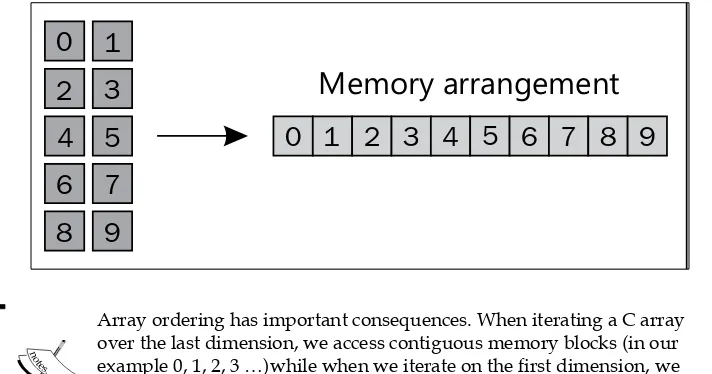
NumPy works as a framework that allows coding complex operations using a concise syntax. The multidimensional array (numpy.ndarray) is internally based on C arrays: in this way, the developer can easily interface NumPy with existing C and FORTRAN code. NumPy constitutes a bridge between Python and the legacy code written using those languages.
In this chapter, we will learn how to create and manipulate NumPy arrays. We will also explore the NumPy broadcasting feature to rewrite complex mathematical expressions in an efficient and succinct manner.
In the last few years a number of packages were developed to further increase the speed of NumPy. We will explore one of these packages, numexpr, that optimizes array expressions and takes advantage of multi-core architectures.
Getting started with NumPy
NumPy is founded around its multidimensional array object, numpy.ndarray. NumPy arrays are a collection of elements of the same data type; this fundamental restriction allows NumPy to pack the data in an efficient way. By storing the data in this way NumPy can handle arithmetic and mathematical operations at high speed.
Creating arrays
You can create NumPy arrays using the numpy.array function. It takes a list-like object (or another array) as input and, optionally, a string expressing its data type. You can interactively test the array creation using an IPython shell as follows:
In [1]: import numpy as np In [2]: a = np.array([0, 1, 2])
Every NumPy array has a data type that can be accessed by the dtype attribute, as shown in the following code. In the following code example, dtype is a 64-bit integer:
In [3]: a.dtype
Out[3]: dtype('int64')
If we want those numbers to be treated as a float type of variable, we can either pass the dtype argument in the np.array function or cast the array to another data type using the astype method, as shown in the following code:
In [4]: a = np.array([1, 2, 3], dtype='float32') In [5]: a.astype('float32')
Out[5]: array([ 0., 1., 2.], dtype=float32)
To create an array with two dimensions (an array of arrays) we can initialize the array using a nested sequence, shown as follows:
In [6]: a = np.array([[0, 1, 2], [3, 4, 5]]) In [7]: print(a)
Out[7]: [[0 1 2] [3 4 5]]
The array created in this way has two dimensions—axes in NumPy's jargon. Such an
array is like a table that contains two rows and three columns. We can access the axes structure using the ndarray.shape attribute:
[ 33 ]
Arrays can also be reshaped, only as long as the product of the shape dimensions is equal to the total number of elements in the array. For example, we can reshape an array containing 16 elements in the following ways: (2, 8), (4, 4), or (2, 2, 4). To reshape an array, we can either use the ndarray.reshape method or directly change the ndarray.shape attribute. The following code illustrates the use of the ndarray. reshape method:
In [7]: a = np.array([0, 1, 2, 3, 4, 5, 6, 7, 8, 9, 10, 11, 12, 13, 14, 15]) In [7]: a.shape
Out[7]: (16,)
In [8]: a.reshape(4, 4) # Equivalent: a.shape = (4, 4) Out[8]:
array([[ 0, 1, 2, 3], [ 4, 5, 6, 7], [ 8, 9, 10, 11], [12, 13, 14, 15]])
Thanks to this property you are also free to add dimensions of size one. You can reshape an array with 16 elements to (16, 1), (1, 16), (16, 1, 1), and so on.
NumPy provides convenience functions, shown in the following code, to create arrays filled with zeros, filled with ones, or without an initialization value (empty— their actual value is meaningless and depends on the memory state). Those functions take the array shape as a tuple and optionally its dtype:
In [8]: np.zeros((3, 3)) In [9]: np.empty((3, 3))
In [10]: np.ones((3, 3), dtype='float32')
In our examples, we will use the numpy.random module to generate random floating point numbers in the (0, 1) interval. In the following code we use the np.random. rand function to generate an array of random numbers of shape (3, 3):
In [11]: np.random.rand(3, 3)
Sometimes, it is convenient to initialize arrays that have a similar shape to other arrays. Again, NumPy provides some handy functions for that purpose such as zeros_like, empty_like, and ones_like. These functions are as follows:
Accessing arrays
The NumPy array interface is, on a shallow level, similar to Python lists. They can be indexed using integers, and can also be iterated using a for loop. The following code shows how to index and iterate an array:
In [15]: A = np.array([0, 1, 2, 3, 4, 5, 6, 7, 8]) In [16]: A[0]
Out[16]: 0
In [17]: [a for a in A]
Out[17]: [0, 1, 2, 3, 4, 5, 6, 7, 8]
It is also possible to index an array in multiple dimensions. If we take a (3, 3) array (an array containing 3 triplets) and we index the first element, we obtain the first triplet shown as follows:
In [18]: A = np.array([[0, 1, 2], [3, 4, 5], [6, 7, 8]]) In [19]: A[0]
Out[19]: array([0, 1, 2])
We can index the triplet again by adding the other index separated by a comma. To get the second element of the first triplet we can index using [0, 1], as shown in the following code:
In [20]: A[0, 1] Out[20]: 1
NumPy allows you to slice arrays in single and multiple dimensions. If we index on the first dimension we will get a collection of triplets shown as follows:
In [21]: A[0:2]
Out[21]: array([[0, 1, 2], [3, 4, 5]])
If we slice the array with [0:2]. for every selected triplet we extract the first two elements, resulting in a (2, 2) array shown in the following code:
In [22]: A[0:2, 0:2] Out[22]: array([[0, 1], [3, 4]])
Intuitively, you can update values in the array by using both numerical indexes and slices. The syntax is as follows:
In [23]: A[0, 1] = 8
[ 35 ]
Indexing with the slicing syntax is fast because it doesn't make copies of
the array. In NumPy terminology it returns a view over the same memory area. If we take a slice of the original array and then change one of its values; the original array will be updated as well. The following code illustrates an example of the same:
In [25]: a = np.array([1, 1, 1, 1]) In [26]: a_view = a[0:2]
In [27]: a_view[0] = 2 In [28]: print(a) Out[28]: [2 1 1 1]
We can take a look at another example that shows how the slicing syntax can be used in a real-world scenario. We define an array r_i, shown in the following line of code, which contains a set of 10 coordinates (x, y); its shape will be (10, 2):
In [29]: r_i = np.random.rand(10, 2)
A typical operation is extracting the x component of each coordinate. In other words, you want to extract the items [0, 0], [1, 0], [2, 0], and so on, resulting in an array with shape (10,). It is helpful to think that the first index is moving while the second one is
fixed (at 0). With this in mind, we will slice every index on the first axis (the moving one) and take the first element (the fixed one) on the second axis, as shown in the following line of code:
In [30]: x_i = r_i[:, 0]
On the other hand, the following expression of code will keep the first index fixed and the second index moving, giving the first (x, y) coordinate:
In [31]: r_0 = r_i[0, :]
Slicing all the indexes over the last axis is optional; using r_i[0] has the same effect as r_i[0, :].
NumPy allows to index an array by using another NumPy array made of either integer or Boolean values—a feature called fancy indexing.
If you index with an array of integers, NumPy will interpret the integers as indexes and will return an array containing their corresponding values. If we index an array containing 10 elements with [0, 2, 3], we obtain an array of size 3 containing the elements at positions 0, 2 and 3. The following code gives us an illustration of this concept:
In [32]: a = np.array([9, 8, 7, 6, 5, 4, 3, 2, 1, 0]) In [33]: idx = np.array([0, 2, 3])
In [34]: a[idx]
You can use fancy indexing on multiple dimensions by passing an array for each dimension. If we want to extract the elements [0, 2] and [1, 3] we have to pack all the indexes acting on the first axis in one array, and the ones acting on the second axis in another. This can be seen in the following code:
In [35]: a = np.array([[0, 1, 2], [3, 4, 5], [6, 7, 8], [9, 10, 11]]) In [36]: idx1 = np.array([0, 1])
In [37]: idx2 = np.array([2, 3]) In [38]: a[idx1, idx2]
You can also use normal lists as index arrays, but not tuples. For example the following two statements are equivalent:
>>> a[np.array([0, 1])] # is equivalent to >>> a[[0, 1]]
However, if you use a tuple, NumPy will interpret the following statement as an index on multiple dimensions:
>>> a[(0, 1)] # is equivalent to >>> a[0, 1]
The index arrays are not required to be one-dimensional; we can extract elements from the original array in any shape. For example we can select elements from the original array to form a (2, 2) array shown as follows:
In [39]: idx1 = [[0, 1], [3, 2]] In [40]: idx2 = [[0, 2], [1, 1]] In [41]: a[idx1, idx2]
Out[41]: array([[ 0, 5], [10, 7]])
The array slicing and fancy indexing features can be combined. For example, this is useful if we want to swap the x and y columns in a coordinate array. In the following code, the first index will be running over all the elements (a slice), and for each of those we extract the element in position 1 (the y) first and then the one in position 0 (the x):
In [42]: r_i = np.random(10, 2)
[ 37 ]
When the index array is a boolean there are slightly different rules. The Boolean array will act like a mask; every element corresponding to True will be extracted and put in the output array. This procedure is shown as follows:
In [44]: a = np.array([0, 1, 2, 3, 4, 5])
In [45]: mask = np.array([True, False, True, False, False, False]) In [46]: a[mask]
Out[46]: array([0, 2])
The same rules apply when dealing with multiple dimensions. Furthermore, if the index array has the same shape as the original array, the elements corresponding to True will be selected and put in the resulting array.
Indexing in NumPy is a reasonably fast operation. Anyway, when speed is critical, you can use the slightly faster numpy.take and numpy.compress functions to squeeze out a little more speed. The first argument of numpy.take is the array we want to operate on, and the second is the list of indexes we want to extract. The last argument is axis; if not provided, the indexes will act on the flattened array, otherwise they will act along the specified axis. The following code shows the use of np.take and its execution time compared to fancy indexing:
In [47]: r_i = np.random(100, 2)
In [48]: idx = np.arange(50) # integers 0 to 50 In [49]: %timeit np.take(r_i, idx, axis=0) 1000000 loops, best of 3: 962 ns per loop In [50]: %timeit r_i[idx]
100000 loops, best of 3: 3.09 us per loop
The similar, but a faster way to index using Boolean arrays is numpy.compress which works in the same way as numpy.take. The use of numpy.compress is shown as follows:
In [51]: idx = np.ones(100, dtype='bool') # all True values In [52]: %timeit np.compress(idx, r_i, axis=0)
1000000 loops, best of 3: 1.65 us per loop In [53]: %timeit r_i[idx]
100000 loops, best of 3: 5.47 us per loop
Broadcasting
Whenever you do an arithmetic operation on two arrays (like a product), if the two operands have the same shape, the operation will be applied in an element-wise fashion. For example, upon multiplying two (2, 2) arrays, the operation will be done between pairs of corresponding elements, producing another (2, 2) array, as shown in the following code:
If the shapes of the operand don't match, NumPy will attempt to match them using certain rules—a feature called broadcasting. If one of the operands is a single value, it will be applied to every element of the array, as shown in the following code:
In [57]: A * 2
Out[58]: array([[2, 4], [6, 8]])
If the operand is another array, NumPy will try to match the shapes starting from the last axis. For example, if we want to combine an array of shape (3, 2) with one of shape (2,), the second array is repeated three times to generate a (3, 2) array. The array is broadcasted to match the shape of the other operand, as shown in the following figure:
If the shapes mismatch, for example by combining an array (3, 2) with an array (2, 2), NumPy will throw an exception.
If one of the axes size is 1, the array will be repeated over this axis until the shapes match. To illustrate that point, if we have an array of the following shape:
5, 10, 2
and we want to broadcast it with an array (5, 1, 2), the array will be repeated on the second axis for 10 times which is shown as follows:
5, 10, 2
5, 1, 2 → repeated
[ 39 ]
We have seen earlier, that we can freely reshape arrays to add axes of size 1. Using the numpy.newaxis constant while indexing will introduce an extra dimension. For instance, if we have a (5, 2) array and we want to combine it with one of shape (5, 10, 2), we could add an extra axis in the middle, as shown in the following code, to obtain a compatible (5, 1, 2) array:
In [59]: A = np.random.rand(5, 10, 2) In [60]: B = np.random.rand(5, 2) In [61]: A * B[:, np.newaxis, :]
This feature can be used, for example, to operate on all possible combinations of the two arrays. One of these applications is the outer product. If we have the following two arrays:
a = [a1, a2, a3] b = [b1, b2, b3]
The outer product is a matrix containing the product of all the possible combinations (i, j) of the two array elements, as shown in the following code:
a x b = a1*b1, a1*b2, a1*b3 a2*b1, a2*b2, a2*b3 a3*b1, a3*b2, a3*b3
To calculate this using NumPy we will repeat the elements [a1, a2, a3] in one dimension, the elements [b1, b2, b3] in another dimension, and then take their product, as shown in the following figure:.
b1 dimensions and get multiplied together using the following code:
AB = a[:, np.newaxis] * b[np.newaxis, :]
Mathematical operations
NumPy includes the most common mathematical operations available for
broadcasting, by default, ranging from simple algebra to trigonometry, rounding, and logic. For instance, to take the square root of every element in the array we can use the numpy.sqrt function, as shown in the following code:
In [59]: np.sqrt(np.array([4, 9, 16])) Out[59]: array([2., 3., 4.])
The comparison operators are extremely useful when trying to filter certain elements based on a condition. Imagine that we have an array of random numbers in the range [0, 1] and we want to extract the numbers greater than 0.5. We can use the > operator on the array; The result will be a boolean array, shown as follows:
In [60]: a = np.random.rand(5, 3) In [61]: a > 0.5
Out[61]: array([[ True, False, True], [ True, True, True], [False, True, True], [ True, True, False],
[ True, True, False]], dtype=bool)
The resulting boolean array can then be reused as an index to retrieve the elements greater than 0.5, as shown in the following code:
In [62]: a[a > 0.5] In [63]: print(a[a>0.5])
[ 0.9755 0.5977 0.8287 0.6214 0.5669 0.9553 0.5894 0.7196 0.9200 0.5781 0.8281 ]
NumPy also implements methods such as ndarray.sum, which takes the sum of all the elements on an axis. If we have an array (5, 3), we can use the ndarray.sum method, as follows, to add elements on the first axis, the second axis, or over all the elements of the array:
In [64]: a = np.random.rand(5, 3) In [65]: a.sum(axis=0)
Out[65]: array([ 2.7454, 2.5517, 2.0303]) In [66]: a.sum(axis=1)
Out[66]: array([ 1.7498, 1.2491, 1.8151, 1.9320, 0.5814]) In [67]: a.sum() # With no argument operates on flattened array Out[67]: 7.3275
[ 41 ]
Calculating the Norm
We can review the basic concepts illustrated in this section by calculating the Norm of a set of coordinates. For a two-dimensional vector the norm is defined as:
norm = sqrt(x^2 + y^2)
Given an array of 10 coordinates (x, y) we want to find the Norm of each coordinate. We can calculate the norm by taking these steps:
1. Square the coordinates: obtaining an array which contains (x**2, y**2) elements.
2. Sum those using numpy.sum over the last axis.
3. Take the square root, element-wise, using numpy.sqrt. The final expression can be compressed in a single line:
In [68]: r_i = np.random.rand(10, 2)
In [69]: norm = np.sqrt((r_i ** 2).sum(axis=1)) In [70]: print(norm)
[ 0.7314 0.9050 0.5063 0.2553 0.0778 0.9143 1.3245 0.9486 1.010 1.0212]
Rewriting the particle simulator in NumPy
In this section, we will optimize our particle simulator by rewriting someparts of it in NumPy. From the profiling we did in Chapter 1, Benchmarking and
Profiling, the slowest part of our program is the following loop contained in the ParticleSimulator.evolve method:
for i in range(nsteps): for p in self.particles:
norm = (p.x**2 + p.y**2)**0.5 v_x = (-p.y)/norm
v_y = p.x/norm
d_x = timestep * p.ang_speed * v_x d_y = timestep * p.ang_speed * v_y
p.x += d_x p.y += d_y
We may notice that the body of the loop acts solely on the current particle. If we had an array containing the particle positions and angular speed, we could rewrite the loop using a broadcasted operation. In contrast, the loop over the time steps depends on the previous step and cannot be treated in a parallel fashion.
It's natural then, to store all the array coordinates in an array of shape (nparticles, 2) and the angular speed in an array of shape (nparticles,). We'll call those arrays r_i and ang_speed_i and initialize them using the following code:
r_i = np.array([[p.x, p.y] for p in self.particles])
ang_speed_i = np.array([p.ang_speed for p in self.particles]) The velocity direction, perpendicular to the vector (x, y), was defined as:
v_x = -y / norm v_y = x / norm
The Norm can be calculated using the strategy illustrated in the Calculating the Norm section under the Getting Started with NumPy heading. The final expression is shown in the following line of code:
norm_i = ((r_i ** 2).sum(axis=1))**0.5
For the components (-y, x) we need first to swap the x and y columns in r_i and then multiply the first column by -1, as shown in the following code:
v_i = r_i[:, [1, 0]] / norm_i v_i[:, 0] *= -1
To calculate the displacement we need to compute the product of v_i, ang_speed_i, and timestep. Since ang_speed_i is of shape (nparticles,) it needs a new axis in order to operate with v_i of shape (nparticles, 2). We will do that using numpy.newaxis constant as follows:
d_i = timestep * ang_speed_i[:, np.newaxis] * v_i r_i += d_i
Outside the loop, we have to update the particle instances with the new coordinates x and y as follows:
[ 43 ]
To summarize, we will implement a method called ParticleSimulator. evolve_numpy and benchmark it against the pure Python version, renamed as ParticleSimulator.evolve_python. The complete ParticleSimulator. evolve_numpy method is shown in the following code:
def evolve_numpy(self, dt): timestep = 0.00001
nsteps = int(dt/timestep)
r_i = np.array([[p.x, p.y] for p in self.particles])
ang_speed_i = np.array([p.ang_speed for p in self.particles])
for i in range(nsteps):
norm_i = np.sqrt((r_i ** 2).sum(axis=1)) v_i = r_i[:, [1, 0]]
v_i[:, 0] *= -1
v_i /= norm_i[:, np.newaxis]
d_i = timestep * ang_speed_i[:, np.newaxis] * v_i r_i += d_i
for i, p in enumerate(self.particles): p.x, p.y = r_i[i]
We also update the benchmark to conveniently change the number of particles and the simulation method as follows:
def benchmark(npart=100, method='python'): particles = [Particle(uniform(-1.0, 1.0), uniform(-1.0, 1.0),
uniform(-1.0, 1.0)) for i in range(npart)]
simulator = ParticleSimulator(particles)
if method=='python':
simulator.evolve_python(0.1)