Advances in Data Mining. Applications and Theoretical Aspects

(1)

Petra Perner (Ed.)

123

LNAI 10933

18th Industrial Conference, ICDM 2018

New York, NY, USA, July 11–12, 2018

Proceedings

Advances in Data Mining

(2)

Lecture Notes in Arti

_ﬁ

cial Intelligence

10933

Subseries of Lecture Notes in Computer Science

LNAI Series Editors

Randy Goebel

University of Alberta, Edmonton, Canada Yuzuru Tanaka

Hokkaido University, Sapporo, Japan Wolfgang Wahlster

DFKI and Saarland University, Saarbrü_{cken, Germany}

LNAI Founding Series Editor

Joerg Siekmann

(3)

(4)

Petra Perner (Ed.)

Advances in Data Mining

Applications and Theoretical Aspects

18th Industrial Conference, ICDM 2018

New York, NY, USA, July 11

_–

12, 2018

Proceedings

(5)

Editor Petra Perner

Institute of Computer Vision and Applied Computer Sciences

Leipzig Germany

ISSN 0302-9743 ISSN 1611-3349 (electronic) Lecture Notes in Artiﬁcial Intelligence

ISBN 978-3-319-95785-2 ISBN 978-3-319-95786-9 (eBook) https://doi.org/10.1007/978-3-319-95786-9

Library of Congress Control Number: 2018947574 LNCS Sublibrary: SL7–Artiﬁcial Intelligence

©_{Springer International Publishing AG, part of Springer Nature 2018}

This work is subject to copyright. All rights are reserved by the Publisher, whether the whole or part of the material is concerned, speciﬁcally the rights of translation, reprinting, reuse of illustrations, recitation, broadcasting, reproduction on microﬁlms or in any other physical way, and transmission or information storage and retrieval, electronic adaptation, computer software, or by similar or dissimilar methodology now known or hereafter developed.

The use of general descriptive names, registered names, trademarks, service marks, etc. in this publication does not imply, even in the absence of a speciﬁc statement, that such names are exempt from the relevant protective laws and regulations and therefore free for general use.

The publisher, the authors and the editors are safe to assume that the advice and information in this book are believed to be true and accurate at the date of publication. Neither the publisher nor the authors or the editors give a warranty, express or implied, with respect to the material contained herein or for any errors or omissions that may have been made. The publisher remains neutral with regard to jurisdictional claims in published maps and institutional afﬁliations.

Printed on acid-free paper

This Springer imprint is published by the registered company Springer International Publishing AG part of Springer Nature

(6)

Preface

The 18th event of the Industrial Conference on Data Mining ICDM was held in New York again (www.data-mining-forum.de) under the umbrella of the World Congress on Frontiers in Intelligent Data and Signal Analysis, DSA 2018 (www.worldcongressdsa.com).

After the peer-review process, we accepted 25 high-quality papers for oral pre-sentation. The topics range from theoretical aspects of data mining to applications of data mining, such as in multimedia data, in marketing, in medicine and agriculture, and in process control, industry, and society. Extended versions of selected papers will appear in the international journalTransactions on Machine Learning and Data Mining (www.ibai-publishing.org/journal/mldm).

In all, 20 papers were selected for poster presentations and six for industry paper presentations, which are published in the ICDM Poster and Industry Proceedings by ibai-publishing (www.ibai-publishing.org).

The tutorial days rounded up the high quality of the conference. Researchers and practitioners got an excellent insight in the research and technology of the respective ﬁelds, the new trends, and the open research problems that we would like to study further.

A tutorial on Data Mining, a tutorial on Case-Based Reasoning, a tutorial on Intelligent Image Interpretation and Computer Vision in Medicine, Biotechnology, Chemistry and Food Industry, and a tutorial on Standardization in Immunofluorescence were held before and in between the conferences of DSA 2018.

We would like to thank all reviewers for their highly professional work and their effort in reviewing the papers.

We also thank the members of the Institute of Applied Computer Sciences, Leipzig, Germany (www.ibai-institut.de), who handled the conference as secretariat. We appreciate the help and understanding of the editorial staff at Springer, and in particular Alfred Hofmann, who supported the publication of these proceedings in the LNAI series.

Last, but not least, we wish to thank all the speakers and participants who contributed to the success of the conference. We hope to see you in 2019 in New York at the next World Congress on Frontiers in Intelligent Data and Signal Analysis, DSA 2019 (www.worldcongressdsa.com), which combines under its roof the following three events: International Conferences Machine Learning and Data Mining, MLDM (www. mldm.de), the Industrial Conference on Data Mining, ICDM (www.data-mining-forum. de), and the International Conference on Mass Data Analysis of Signals and Images in Medicine, Biotechnology, Chemistry, Biometry, Security, Agriculture, Drug Discovery and Food Industry, MDA (www.mda-signals.de), as well as the workshops, and tutorials.

(7)

Organization

Chair

Petra Perner IBaI Leipzig, Germany

Program Committee

Ajith Abraham Machine Intelligence Research Labs (MIR Labs), USA Brigitte Bartsch-Spö_rl _{BSR Consulting GmbH, Germany}

Orlando Belo University of Minho, Portugal Bernard Chen University of Central Arkansas, USA Antonio Dourado University of Coimbra, Portugal Jeroen de Bruin Medical University of Vienna, Austria Stefano Ferilli University of Bari, Italy

Geert Gins KU Leuven, Belgium

Warwick Graco ATO, Australia

Aleksandra Gruca Silesian University of Technology, Poland Hartmut Ilgner Council for Scientiﬁc and Industrial Research,

South Africa

Pedro Isaias Universidade Aberta (Portuguese Open University), Portugal

Piotr Jedrzejowicz Gdynia Maritime University, Poland Martti Juhola University of Tampere, Finland Janusz Kacprzyk Polish Academy of Sciences, Poland Mehmed Kantardzic University of Louisville, USA

Eduardo F. Morales INAOE, Ciencias Computacionales, Mexico Samuel Noriega Universitat de Barcelona Spain

Juliane Perner Cancer Research, Cambridge Institutes, UK Armand Prieditris Newstar Labs, USA

Rainer Schmidt University of Rostock, Germany Victor Sheng University of Central Arkansas, USA

Kaoru Shimada Section of Medical Statistics, Fukuoka Dental College, Japan

(8)

Additional Reviewers

(9)

An Adaptive Oversampling Technique

for Imbalanced Datasets

Shaukat Ali Shahee and Usha Ananthakumar(B)

Indian Institute of Technology Bombay, Mumbai 400076, India [email protected],[email protected]

Abstract. Class imbalance is one of the challenging problems in classifi-cation domain of data mining. This is particularly so because of the inabil-ity of the classifiers in classifying minorinabil-ity examples correctly when data is imbalanced. Further, the performance of the classifiers gets deteriorated due to the presence of imbalance within class in addition to between class imbalance. Though class imbalance has been well addressed in literature, not enough attention has been given to within class imbalance. In this paper, we propose a method that can adaptively handle both between-class and within-between-class imbalance simultaneously and also that can take into account the spread of the data in the feature space. We validate our approach using 12 publicly available datasets and compare the clas-sification performance with other existing oversampling techniques. The experimental results demonstrate that the proposed method is statisti-cally superior to other methods in terms of various accuracy measures.

Keywords: Classification

·

Imbalanced dataset

·

Oversampling Model based clustering

·

Lowner John ellipsoid

1 Introduction

In data mining literature, class imbalance problem is considered to be quite challenging. The problem arises when the class of interest contains a relatively lower number of examples compared to other class examples. In this study, the minority class, the class of interest is considered positive and the majority class is considered negative. Recently, several authors have addressed this problem in various real life domains including customer churn prediction [6], financial distress prediction [10], employee churn prediction [39], gene regulatory network reconstruction [7] and information retrieval and filtering [35]. Previous studies have shown that applying classifiers directly to imbalance dataset results in poor performance [34,41,43]. One of the possible reasons for the poor performance is skewed class distribution because of which the classification error gets dominated by the majority class. Another kind of imbalance is referred to as within-class imbalance which pertains to the state where a class composes of different number of sub-clusters (sub-concepts) and these sub-clusters in turn, containing different number of examples.

c

Springer International Publishing AG, part of Springer Nature 2018 P. Perner (Ed.): ICDM 2018, LNAI 10933, pp. 1–16, 2018.

(12)

2 S. A. Shahee and U. Ananthakumar

In addition to class imbalance, small disjuncts, lack of density, overlapping between classesandnoisy examplesalso deteriorate the performance of the clas-sifiers [2,28–30,36]. Thebetween-class imbalance along withwithin-class imbal-ance is an instimbal-ance of problem of small disjuncts [26]. Literature presents dif-ferent ways of handling class imbalance such as data preprocessing, algorithmic based, cost-based methods and ensemble of classifier sampling methods [12,17]. Though no method is superior in handling all imbalanced problems, sampling based methods have shown great capability as they attempt to improve data distribution rather than the classifier [3,8,23,42]. Sampling method is a prepro-cessing technique that modifies the imbalanced data to a balanced data using some mechanism. This is generally carried out by either increasing the minority class examples called as oversampling or by decreasing the majority examples, referred to as undersampling [4,13]. It is not advisable to undersample the major-ity class examples if minormajor-ity class has complete rarmajor-ity [40]. The current literature available on simultaneousbetween-classimbalance andwithin-classimbalance is limited.

In this paper, an adaptive method for handling between class imbalance and within class imbalance simultaneously based on an oversampling technique is proposed. It also factors in the scatter of data for improving the accuracy of both the classes on the test set. Removing between class imbalance and within class imbalance simultaneously helps the classifier to give equal importance to all the sub-clusters, and adaptively increasing the size of sub-clusters handles the randomness in the dataset. Generally, classifier minimizes the total error, and removal of between class imbalance and within class imbalance helps the classifier in giving equal weight to all the sub-clusters irrespective of the classes thus resulting in increased accuracy of both the classes. Neural network is one such classifier and is being used in this study. The proposed method is validated on publicly available data sets and compared with well known existing oversampling techniques. Section2 discusses the proposed method and analysis on publicly available data sets is presented in Sect.3. Finally, Sect.4 concludes the paper with future work.

2 An Adaptive Oversampling Technique

The approach in this proposed method is to oversample the examples in such a way that it helps the classifier in increasing the classification accuracy on the test set.

The proposed method is based on two challenging aspects faced by the clas-sifiers in case of imbalanced data sets. First one is the case of the loss function, where the majority class dominates the minority class and thus eventually, min-imization of the loss function is largely due to minmin-imization of the majority class. Because of this, the decision boundary between the classes does not get shifted towards the minority class. Removing the between class and within class imbalance helps in removing the dominance of the majority class.

(13)

An Adaptive Oversampling Technique for Imbalanced Datasets 3

Fig. 1.Synthetic minority class examples generation on the peripheral of Lowner John ellipsoids

outskirts of the sub-clusters, there is a need to adjust the decision boundary to minimize misclassification. This is achieved by expanding the size of the sub-cluster in order to cope with such test examples. Now the question is, what is the surface of the sub-clusters and how far the sub-clusters should be expanded. To answer this, we use minimum volume ellipsoid that contains the dataset known as Lowner John ellipsoid [33]. We adaptively increase the size of the ellipsoid and synthetic examples are generated on the surface of the ellipsoid. One such instance is shown in Fig.1 where minority class examples are denoted by stars and majority class examples by circle.

In the proposed method, the first step is data cleaning where the noisy exam-ples are removed from the dataset as this helps in reducing the oversampling of noisy examples. After data cleaning, the concept is detected by using model based clustering and the boundary of each of the clusters is determined by Lowner John ellipsoid. Subsequently, the number of examples to be oversam-pled is determined based on the complexity of sub-clusters and synthetic data are generated on the peripheral of the ellipsoid. Following section elaborates the proposed method in detail.

2.1 Data Cleaning

(14)

2.2 Locating Sub-clusters

Model based clustering [16] is used with respect to minority class to identify the sub-clusters (or sub-concepts) present in the dataset. We have used MCLUST [15] for implementing the model based clustering. MCLUST is aRpackage that implements the combination of hierarchical agglomerative clustering, Expecta-tion MaximizaExpecta-tion (EM) and Bayesian InformaExpecta-tion criterion (BIC) for compre-hensive cluster analysis.

2.3 Structure of Sub-clusters

The structure of sub-clusters can be obtained using eigenvalues and eigenvector. Eigenvectors gives the shape of sub-cluster and size is given by eigenvalues. Let X ={x1, x2, . . . , xm} be a dataset having m examples andn features. Let the

mean vector of X be µ and the covariance matrix computed by Σ = E[(X− µ)(X−µ)T_{]. The eigenvalues (}_λ_{) and eigenvectors}_v_{of the covariance matrix}_Σ

are found such thatΣv=λv.

2.4 Identifying the Boundary of Sub-clusters

For each of the sub-clusters, Lowner-John ellipsoid is obtained as given by [33]. This is a minimum volume ellipsoid that contains the convex hull of C={x1, x2, . . . , xm} ⊆Rn. The general equation of ellipsoid is

ε={v|||Av+b||2≤1} (1)

We assume that A ∈ Sn

++ is a positive definite matrix where the volume of ε is proportional to detA−1_{. The problem of computing the minimum volume} ellipsoid containing C can be expressed as

minimize logdetA−1

subject to ||Axi+b||2≤1, i= 1, . . . , m. (2)

We useCVX [21], a Matlab-based modeling system for solving this optimization problem.

2.5 Synthetic Data Generation

The synthetic data generation is based on the following three steps

1. In the first step, the proposed method determines the number of examples to be oversampled per cluster. The number of minority class examples to be oversampled is computed using Eq. (3).

N =T C0−T C1 (3)

(15)

It then computes the complexity of sub-clusters based on the number of dan-ger zone examples. An example is called a dandan-ger zone example or a borderline example if an example under consideration is surrounded by more than 50% examples of other class as also being considered in other studies including [23]. That is, ifk is the number of nearest neighbors under consideration, an example being a danger zone example implies k/2 ≤ z < k where z is the number of other class examples among thek nearest neighbor examples. For example, Fig.2shows two sub-clusters of minority class having 4 and 2 danger zone examples. In this study, we considerk= 5 as in [3]. Letc1, c2, c3, . . . , cq

be the number of danger zone examples present in the sub-clusters 1,2, . . . , q respectively. The number of examples to be oversampled in the sub-clusteri is given by

2. Having determined the number of examples to be oversampled, the next task is to weigh the danger zone examples in accordance with the direction of the ellipsoid and its distance from the centroid. These weights are computed with respect to the eigenvectors of the variance-covariance matrix of the dataset. For example, consider Fig.3whereAandBdenote the danger zone examples. Here we compute the inner product between danger zone examples A and B with the eigenvectors Evec1 and EVec2 that form acute angles with the danger zone examples. The weight ofA,W(A) is computed as

W(A) =A, EV ec1+A, Evec2 (5)

Similarly the weight ofB,W(B) is computed as

W(B) =B, EV ec1+B, Evec2 (6)

Thus, when data is n dimensional, the total weight of the bth

k danger zone

whereei is the eigenvector.

3. In each of the sub-clusters, synthetic examples are generated on theLowner John ellipsoid by linear extrapolation of the selected danger zone example where the selection of danger zone example is carried out with respect to the weights obtained in step 2. Here

P(bk) =

wk

ci

i=1wi

(8)

where P(bk) is the probability of selecting danger zone example bk and

wk is the weight of kth danger zone example present in the sub-cluster ci.

(16)

Fig. 2.Illustration of danger zone examples of minority class sub-clusters extrapolated vector withLowner John ellipsoid. Let the centroid of the ellip-soid becenter=−A−1_∗_b_{and if}_b_k_{is the danger zone example selected based} on the probability distribution given by Eq. (8), the vector v =bk −center

is extrapolated by ‘r’ units to intersect with the ellipsoid and the synthetic examplestthus generated is given by

st=center+

(r+C)∗v

v (9)

whereCcontrols the expansion of the ellipsoid.

(17)

The whole procedure of the algorithm is explained in Algorithm1.

Algorithm 1.An Adaptive Oversampling Technique for Imbalanced Data sets Input: Training dataset:S ={Xi, yi}, i= 1, ..., m;Xi∈Rn _and_yi_{∈ {}₀_,₁_}_Positive

2: Apply Model-Based clustering onS+, return{smin1, ...sminq}sub-clusters. 3: foreach minority sub-cluster smini, 1≤i≤q do

4: Bi←DangerzoneExample₍_smini_{) //Return list of danger zone examples} 5: end for

12: Compute the Lowner John ellipsoids ofsmini as given in Subsect. 2.4 givesA andb

13: The eigenvectorsv1, ..., vnand eigenvaluesλ1, ...λnof the covariance matrixΣi of dataset in sub-clusterssmini is computed byΣvi=λiv

14: forj= 1 to length(Bi)do

// Compute the prob. dist of danger zone examples

25: N ewSyntheticExample=Φ 26: fort= 1 to nido

27: Select the danger zone example basedbibased on step 24 28: Synthetic examplesthas been generated as given in equation (9) 29: N ewSyntheticExample=N ewSyntheticExample∪ {st} 30: end for

(18)

3 Experiments

3.1 Data Sets

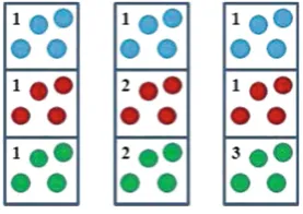
We evaluate the proposed method on 12 publicly available datasets which have skewed class distribution available on the KEEL dataset [1] repository. Asyeast andpageblocks data sets have multiple classes, we have suitably transformed the data sets to two classes to meet our needs of binary class problem. In case of yeast dataset, it has 1484 examples and 10 classes {MIT, NUC, CYT, ME1, ME2, ME3, EXC, VAC, POX, ERL}. We choose ME3 as the minority class and the remaining are combined to form the majority class. In case ofpageblocks dataset, it has 548 examples and 5 classes{1, 2, 3, 4, 5}. We choose1 as majority class and the rest as the minority class. Minority class is chosen in both the data sets in such a way that it contains reasonable number of examples to identify the presence of sub-concepts and also to maintain the imbalance with respect to the majority class. The rest of the data sets were taken as they are. Table1 represents the characteristics of various data sets used in the analysis.

Table 1.The data sets

Data sets Total exp Minority exp Majority exp No. attribute

glass1 214 76 138 9

pima 768 268 500 8

glass0 214 70 144 9

yeast1 1484 429 1055 8

vehicle2 846 218 628 18

ecoli1 336 77 259 7

yeast 1484 163 1321 8

glass6 214 29 185 9

yeast3 1484 163 1321 8

yeast-0-5-6-7-9 vs 4 528 51 477 8

yeast-0-2-5-7-9 vs 3-6-8 1004 99 905 8

pageblocks 548 56 492 10

3.2 Assessment Metrics

(19)

An Adaptive Oversampling Technique for Imbalanced Datasets 9 Error rate= 1−Accuracy

(10)

These confusion matrix based measures described by [25] for imbalanced learning problem are precision, recall,F-measure and G-mean. These measures are defined as Here β is a non-negative parameter that controls the influence of precision and recall. In this study, we set β = 1 implying that precision and recall are equally important.

Another popular technique for evaluation of classifiers under imbalance domain is the Receiving Operating Characteristic (ROC) curve [37]. ROC curve is a graphical representation of the performance of the classifier by plottingTP rates versusFP ratesover possible threshold values. The TP rates and FP rates are defined as

TP rate = T P

T P+F N (15)

FP rate = F P

F P +T N (16)

(20)

Fig. 4.Results ofF-measure _{of majority class for various methods with the best one} being highlighted.

3.3 Experimental Settings

In this work, we have used the feed-forward neural network with backpropa-gation. The structure of the network is such that it has input layers with the number of neurons being equal to the number of features. The number of neurons in the output layer is one as it is a binary classification problem. The number of neurons in the hidden layer is the average of the number of features and num-ber of classes [22]. The activation function used at each neuron is the sigmoid function with learning rate 0.3.

We compare our proposed method with well known existing oversampling methods such as SMOTE [8], ADASYN [24], MWMOTE [3] and CBO [30]. We use default parameter settings for these oversampling techniques. In case of SMOTE [8], the number of nearest neighbor kis set to 5. In case ofADASYN [24], the number of nearest neighbor k is 5 and desired level of balance is 1. In case of MWMOTE [3], the number of neighbors used for predicting noisy minority class examples is k1 = 5, the number of nearest neighbors used to find majority class examples isk2 = 3, the percentage of original minority class examples used in generating synthetic examples isk3 =|Smin|/2, the number of clusters in the method isCp= 3 and smoothing and rescaling values of different scaling factors areCf(th) = 5 and CM AX= 2 respectively.

3.4 Results

(21)

Fig. 5.Results of F-measure _{of minority class for various methods with the best one} being highlighted.

Fig. 6.Results ofG-mean _{for various methods with the best one being highlighted.}

combined and considered as the training set. Oversampling is carried out only on the training set and not on the test set in order to obtain unbiased estimates of the model for future prediction.

Figure4shows the results ofF-measureof majority class. It is clear from the figure that the proposed method outperforms the other oversampling methods for different values of C. In this study, we consider C ∈ {0,2,4,6} where C controls the expansion of the ellipsoid.C= 0 gives the minimum volume Lowner-John ellipsoid and C = 2 means the size of ellipsoid increases by 2 units. The results of Fmeasure1 is shown in Fig.5. From the figure it is clear that the proposed method outperforms the other methods except in case of data sets glass1, glass0 andyeast1whereCBO, SMOTE andMWMOTEperform slightly better. Similarly, the results in case of G-mean and AUC are shown in Figs.6 and7 respectively. The method yielding the best result is highlighted in all the figures.

(22)

Fig. 7.Results ofAUC for various methods with the best one being highlighted.

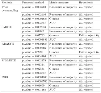
Table 3.Summary of Wilcoxon signed rank test between our proposed method and other methods

Methods Proposed method Metric measure Hypothesis Prior

oversampling

p value = 0.003204 F-measure of majority H0 rejected

p value = 0.002516 F-measure of minority H0 rejected p value = 0.0004883 G-mean H0 rejected

p value = 0.003857 AUC H0 rejected

SMOTE p value = 0.002516 F-measure of majority H0 rejected p value = 0.02061 F-measure of minority H0 rejected p value = 0.07733 G-mean Fail to rejectH0

ADASYN p value = 0.0004883 F-measure of majority H0 rejected p value = 0.009766 F-measure of minority H0 rejected p value = 0.2298 G-mean Fail to rejectH0

MWMOTE p value = 0.002478 F-measure of majority H0 rejected p value = 0.01344 F-measure of minority H0 rejected p value = 0.02531 G-mean H0 rejected

CBO p value = 0.0004883 F-measure of majority H0 rejected p value = 0.0009766 F-measure of minority H0 rejected p value = 0.01669 G-mean H0 rejected

(23)

signed-rank non-parametric test [38] is carried out on F-measure of majority class, F-measure of minority class, G-Mean and AUC. The null and alternative hypothesis are as follows:

H0: The median difference is zero H1: The median difference is positive.

This test computes the difference in the respective measure between the proposed method and the method compared with it and ranks the absolute differences. LetW+ be the sum of the ranks with positive differences andW− be the sum of the ranks with negative differences. The test statistic is defined as W =min(W+, W−). Since there are 12 data sets, theW value should be less than 17 (critical value) at a significance level of 0.05 to reject H0 [38]. Table3 shows thep-values of test statistics of Wilcoxon signed-rank test.

The statistical tests indicate that the proposed method statistically outper-forms the other methods in terms ofAUC andF-measure of both minority and majority class, although in case ofG-mean measure, the proposed method does not seem to outperformSMOTE andADASYN. Since we useAUC for compar-ison purpose, it can be inferred that our proposed method is superior to other oversampling methods.

4 Conclusion

In this paper, we propose an oversampling method that adaptively handles between class imbalance and within class imbalance simultaneously. The method identifies the concepts present in the data set using model based clustering and then eliminates the between class and within class imbalance simultaneously by oversampling the sub-clusters where the number of examples to be oversampled is determined based on the complexity of the sub-clusters. The method focuses on improving the test accuracy by adaptively expanding the size of sub-clusters in order to cope with unseen test data. 12 publicly available data sets were ana-lyzed and the results show that the proposed method outperforms the other methods in terms of different performance measures such asF-measure of both the majority and minority class and AUC.

(24)

References

1. Alcalá, J., Fernández, A., Luengo, J., Derrac, J., Garc´ıa, S., Sánchez, L., Herrera, F.: Keel data-mining software tool: data set repository, integration of algorithms and experimental analysis framework. J. Multiple-Valued Log. Soft Comput.17(2– 3), 255–287 (2010)

2. Alshomrani, S., Bawakid, A., Shim, S.O., Fern´andez, A., Herrera, F.: A proposal for evolutionary fuzzy systems using feature weighting: dealing with overlapping in imbalanced datasets. Knowl.-Based Syst.73, 1–17 (2015)

3. Barua, S., Islam, M.M., Yao, X., Murase, K.: Mwmote-majority weighted minority oversampling technique for imbalanced data set learning. IEEE Trans. Knowl. Data Eng.26(2), 405–425 (2014)

4. Batista, G.E., Prati, R.C., Monard, M.C.: A study of the behavior of several meth-ods for balancing machine learning training data. ACM SIGKDD Explor. Newsl. 6(1), 20–29 (2004)

5. Bradley, A.P.: The use of the area under the ROC curve in the evaluation of machine learning algorithms. Pattern Recogn.30(7), 1145–1159 (1997)

6. Burez, J., Van den Poel, D.: Handling class imbalance in customer churn prediction. Expert Syst. Appl.36(3), 4626–4636 (2009)

7. Ceci, M., Pio, G., Kuzmanovski, V., Dˇzeroski, S.: Semi-supervised multi-view learn-ing for gene network reconstruction. PLoS ONE10(12), e0144031 (2015)

8. Chawla, N.V., Bowyer, K.W., Hall, L.O., Kegelmeyer, W.P.: Smote: synthetic minority over-sampling technique. J. Artif. Intell. Res.16, 321–357 (2002) 9. Chawla, N.V., Lazarevic, A., Hall, L.O., Bowyer, K.W.: SMOTEBoost: improving

prediction of the minority class in boosting. In: Lavraˇc, N., Gamberger, D., Todor-ovski, L., Blockeel, H. (eds.) PKDD 2003. LNCS (LNAI), vol. 2838, pp. 107–119. Springer, Heidelberg (2003).https://doi.org/10.1007/978-3-540-39804-2 12 10. Cleofas-Sánchez, L., Garc´ıa, V., Marqués, A., Sánchez, J.S.: Financial distress

pre-diction using the hybrid associative memory with translation. Appl. Soft Comput. 44, 144–152 (2016)

11. Demˇsar, J.: Statistical comparisons of classifiers over multiple data sets. J. Mach. Learn. Res.7(Jan), 1–30 (2006)

12. D´ıez-Pastor, J.F., Rodr´ıguez, J.J., Garc´ıa-Osorio, C.I., Kuncheva, L.I.: Diversity techniques improve the performance of the best imbalance learning ensembles. Inf. Sci.325, 98–117 (2015)

13. Estabrooks, A., Jo, T., Japkowicz, N.: A multiple resampling method for learning from imbalanced data sets. Comput. Intell.20(1), 18–36 (2004)

14. Fawcett, T.: ROC graphs: notes and practical considerations for researchers. Mach. Learn.31(1), 1–38 (2004)

15. Fraley, C., Raftery, A.E.: MCLUST: software for model-based cluster analysis. J. Classif.16(2), 297–306 (1999)

16. Fraley, C., Raftery, A.E.: Model-based clustering, discriminant analysis, and den-sity estimation. J. Am. Stat. Assoc.97(458), 611–631 (2002)

17. Galar, M., Fernandez, A., Barrenechea, E., Bustince, H., Herrera, F.: A review on ensembles for the class imbalance problem: bagging-, boosting-, and hybrid-based approaches. IEEE Trans. Syst. Man Cybern. Part C (Appl. Rev.)42(4), 463–484 (2012)

(25)

19. Garcia, S., Herrera, F.: An extension on “statistical comparisons of classifiers over multiple data sets” for all pairwise comparisons. J. Mach. Learn. Res. 9(Dec), 2677–2694 (2008)

20. Garc´ıa, V., Mollineda, R.A., S´anchez, J.S.: A bias correction function for classi-fication performance assessment in two-class imbalanced problems. Knowl.-Based Syst.59, 66–74 (2014)

21. Grant, M., Boyd, S., Ye, Y.: CVX: Matlab software for disciplined convex pro-gramming (2008)

22. Guo, H., Viktor, H.L.: Boosting with data generation: improving the classification of hard to learn examples. In: Orchard, B., Yang, C., Ali, M. (eds.) IEA/AIE 2004. LNCS (LNAI), vol. 3029, pp. 1082–1091. Springer, Heidelberg (2004).https://doi. org/10.1007/978-3-540-24677-0 111

23. Han, H., Wang, W.-Y., Mao, B.-H.: Borderline-SMOTE: a new over-sampling method in imbalanced data sets learning. In: Huang, D.-S., Zhang, X.-P., Huang, G.-B. (eds.) ICIC 2005. LNCS, vol. 3644, pp. 878–887. Springer, Heidelberg (2005). https://doi.org/10.1007/11538059 91

24. He, H., Bai, Y., Garcia, E.A., Li, S.: ADASYN: adaptive synthetic sampling app-roach for imbalanced learning. In: IEEE International Joint Conference on Neural Networks, IJCNN 2008, (IEEE World Congress on Computational Intelligence), pp. 1322–1328. IEEE (2008)

25. He, H., Garcia, E.A.: Learning from imbalanced data. IEEE Trans. Knowl. Data Eng.21(9), 1263–1284 (2009)

26. Holte, R.C., Acker, L., Porter, B.W., et al.: Concept learning and the problem of small disjuncts. In: IJCAI, vol. 89, pp. 813–818. Citeseer (1989)

27. Huang, J., Ling, C.X.: Using auc and accuracy in evaluating learning algorithms. IEEE Trans. Knowl. Data Eng.17(3), 299–310 (2005)

28. Japkowicz, N.: Class imbalances: are we focusing on the right issue. In: Workshop on Learning from Imbalanced Data Sets II, vol. 1723, p. 63 (2003)

29. Japkowicz, N., Stephen, S.: The class imbalance problem: a systematic study. Intell. Data Anal.6(5), 429–449 (2002)

30. Jo, T., Japkowicz, N.: Class imbalances versus small disjuncts. ACM SIGKDD Explor. Newsl.6(1), 40–49 (2004)

31. Kubat, M., Matwin, S., et al.: Addressing the curse of imbalanced training sets: one-sided selection. In: ICML, vol. 97, Nashville, USA, pp. 179–186 (1997) 32. Lango, M., Stefanowski, J.: Multi-class and feature selection extensions of roughly

balanced bagging for imbalanced data. J. Intell. Inf. Syst.50(1), 97–127 (2018) 33. Lutwak, E., Yang, D., Zhang, G.:LpJohn ellipsoids. Proc. Lond. Math. Soc.90(2),

497–520 (2005)

34. Maldonado, S., L´opez, J.: Imbalanced data classification using second-order cone programming support vector machines. Pattern Recogn.47(5), 2070–2079 (2014) 35. Piras, L., Giacinto, G.: Synthetic pattern generation for imbalanced learning in

image retrieval. Pattern Recogn. Lett.33(16), 2198–2205 (2012)

36. Prati, R.C., Batista, G.E.A.P.A., Monard, M.C.: Class imbalances versus _class overlapping: an analysis of a learning system behavior. In: Monroy, R., Arroyo-Figueroa, G., Sucar, L.E., Sossa, H. (eds.) MICAI 2004. LNCS (LNAI), vol. 2972, pp. 312–321. Springer, Heidelberg (2004). https://doi.org/10.1007/978-3-540-24694-7 32

(26)

38. Richardson, A.: Nonparametric statistics for non-statisticians: a step-by-step app-roach by Gregory W. Corder, Dale I. Foreman. Int. Stat. Rev. 78(3), 451–452 (2010)

39. Saradhi, V.V., Palshikar, G.K.: Employee churn prediction. Expert Syst. Appl. 38(3), 1999–2006 (2011)

40. Weiss, G.M.: Mining with rarity: a unifying framework. ACM SIGKDD Explor. Newsl.6(1), 7–19 (2004)

41. Yang, C.Y., Yang, J.S., Wang, J.J.: Margin calibration in SVM class-imbalanced learning. Neurocomputing 73(1), 397–411 (2009)

42. Yen, S.J., Lee, Y.S.: Cluster-based under-sampling approaches for imbalanced data distributions. Expert Syst. Appl.36(3), 5718–5727 (2009)

(27)

From Measurements to Knowledge

-Online Quality Monitoring and Smart

Manufacturing

Satu Tamminen1(B)_{, Henna Tiensuu}1_{, Eija Ferreira}1_{, Heli Helaakoski}2_,

Vesa Kyll¨onen2, Juha Jokisaari3, and Esa Puukko4

1

Abstract. The purpose of this study was to develop an innovative supervisor system to assist the operators in an industrial manufactur-ing process to help discover new alternative solutions for improvmanufactur-ing both the products and the manufacturing process.

This paper presents a solution for integrating different types of sta-tistical modelling methods for a usable industrial application in quality monitoring. The two case studies demonstrating the usability of the tool were selected from a steel industry with different needs for knowledge presentation. The usability of the quality monitoring tool was tested in both case studies, both offline and online.

Keywords: Data mining

_·

Smart manufacturing

_·

Online monitoring Quality prediction

_·

Knowledge representation

_·

Machine learning

1 Introduction

Knowledge can be considered to be the most valuable asset of a manufacturing enterprise, when defining itself in the market and competing with others. The competitiveness of today’s industry is built on quality management, delivery reliability and resource efficiency, which are dependent on the effective usage of the data collected from all possible sources. The risk is that the operators with the limited capacity to process the incessant information flow miss the essential knowledge within the data. Recent advances in statistical modelling, machine learning and IT technologies create new opportunities to utilize the industrial data efficiently and to distribute the refined knowledge to end users in right time and convenient format.

Manufacturing has benefited from the field of data mining in several areas, including engineering design, manufacturing systems, decision support systems,

c

Springer International Publishing AG, part of Springer Nature 2018

(28)

18 S. Tamminen et al.

shop floor control and layout, fault detection, quality improvement, maintenance, and customer relationship management [1]. While the amount of data expands rapidly, there is a need for automated and intelligent tools for data mining. Statis-tical regression and classification methods have been utilized for steel plate moni-toring [2]. Decision support systems (DSS), for example, become intelligent when combined with AI tools such as fuzzy logic, case-based reasoning, evolutionary computing, artificial neural networks (ANN), and intelligent agents [3,4].

Knowledge engineering and data mining have enabled the development of new types of manufacturing systems. Future manufacturing is able to adapt to demands of agile manufacturing, including a rapid response to changing customer requirements, concurrent design and engineering, lower cost of small volume pro-duction, outsourcing of supply, distributed manufacturing, just-in-time delivery, real-time planning and scheduling, increased demands for precision and quality, reduced tolerance for errors, in-process measurements and feedback control [5]. Smart manufacturing will bring solutions to existing challenges, but the cur-rent industry utilizes generally the information from its environment and in best cases only the first level of knowledge (Fig.1). The progress in industrial data utilization is enabled with novel intelligent data processing methods.

Fig. 1.The evolution of data to knowledge requires novel methods for intelligent data processing that enable the shift to smart manufacturing.

(29)

From Measurements to Knowledge 19

experts concentrate on the core area of the industry, which in its turn, generate a demand for intelligent tools for decision support.

Information presentation is a complex task in manufacturing, as the amount of quality parameters that need to be linked with even a larger number of pro-cess parameters is difficult to propro-cess with capabilities of a human being. Akram et al._{show how statistical process control (SPC) and automatic process control} (APC) can be integrated for process monitoring and adjustment [8]. Statistical models bring wider possibility to produce information with their capability to predict the future outcome, which enables the process and production planning. The challenge is how to enable the communication between people, how to get information that they need from the process or the product, if the information transfer is enabled between the work posts or manufacturing facilities, or how to provide information about the malfunction or decreased quality of the prod-ucts. The information should be presented clearly, solutions for the problem, also warnings if automatic corrective actions are enabled. As a whole, the infor-mation chain should be supported with a tool that enables the knowledge based conversation within the company.

When product quality improvement is pursued, Kano and Nakagawa suggest that the process monitoring system should have at least the following functions: it should be able to predict product quality from operating conditions, to derive better operating conditions that can improve the product quality, and to detect faults or malfunctions for preventing undesirable operation. They have used soft sensors for quality prediction, optimization for operating conditions improve-ment, and multivariate statistical process control (MSPC) for fault detection in steel industry application [9]. From these objectives, the derivation of better operating conditions may be the most difficult one to reach; even the definition for better conditions can be challenging to draw, as the conditions are often a compromise of least harmful and cost efficient practices.

In this article, we propose a method for online quality monitoring during a manufacturing process with two application cases in steel industry. Our tool links together the statistical models for prediction of quality properties based on the process settings and variables, and presents the results with easily inter-pretable visualisations. This paper is organized as follows. Section2describes the requirements and specifications for online quality monitoring tool for industrial use. Section3 presents the choice of the modelling method for quality moni-toring purposes. The quality prediction based tools for decision support in two case studies are presented in Sect.4. Section5concludes the quality monitoring development.

2 Developing a Quality Monitoring

Tool for Industrial Use

2.1 The Domain Requirements and Requests

(30)

process industry. We arranged a series of workshops with participating compa-nies, development partners and other stakeholders.

When specifying the requirements of the QMT, we selected the key user groups for the first development step. This way, the tool could be demonstrated with users having different needs. The selection had the highest impact on the user interface and information presentation.

Technical specifications of the quality tool were stable and reliable applica-tions, performance, maintainability, scalability: adding new modules, features, methods or algorithms should be easy, security, authentication, recoverability, standards and tools (programming languages) and accessibility (web applica-tion) are also needed.

The QMT prototype is illustrated in Fig.2. The transfer of the information from the manufacturing process to the end users is presented in the following four steps that are (1) data acquisition, (2) data storage, (3) information analysis and (4) information delivery. In most advanced visualizations in our tool, the information has been refined to knowledge with automatic interpretation of the results.

Fig. 2.The prototype of QMT.

2.2 The Specifications for the Tool

The quality information in the QMT is based on the statistical prediction models implemented in R language and equations and rules implemented in C++Mathematical ExpressionToolkit Library (ExprTk). R is a free and open source language for statistical computing. R is integrated into QMT with RServe module, which allows other programs to use facilities of R. R scripts can be writ-ten standalone and integration into QMT is straightforward. ExprTk is a math-ematical expression parsing and evaluation engine. It is integrated into QMT by including it directly to the source code.

(31)

for QMT is accomplished by reading data from a database. Typically, selected database views are created for accessing data from a database. Some data pre-processing is needed before data can be used for model calculation. For example, a valid range for all model input variables has been defined, and if these limits were violated, model result may not be reliable which is shown with a question mark in the QMT user interface.

The QMT user interface is web based, and in typical use, it provides an overview of process quality as a starting point. In the quality overview, colour coded bars present the quality status of different process phases for each product during the selected time span. Typically, red colour indicates process failure or malfunction, yellow a warning for a process failure and green normal operation. Additionally, white colour indicates that quality information could not be calcu-lated for some reason. Figure3 illustrates a screen shot from the user interface. The overview to the process shows the predicted quality based on several quality models at different process steps. It hides mathematical models and all process variables from which the quality information is composed. The user can define the relevant quality models to be presented, and if any specific product looks interesting, the tool provides a possibility to analyse it further just by clicking the corresponding bar. Naturally, different user groups require different kinds of views to QMT based on their needs.

Fig. 3.The user interface of QMT. (Color figure online)

3 Statistical Quality Models

(32)

property. With an online system, the functionality of the tool would suffer, if the models were not capable of processing observations with missing data.

During the last two decades, neural networks have been a popular method for modelling data with complex relations between variables [10–12]. Lately, ensem-ble algorithms have risen to challenge them with equal accuracy, faster learning, tendency to reduce bias and variance, and they are more likely to over-fit. Seni and Elder state that ensemble methods have been called the most influential development in data mining and machine learning in the past decade [13]. Gra-dient boosting machines are a family of powerful machine learning techniques that has been successfully applied to a wide range of practical applications [14]. Boosted regression trees are capable of handling different types of predictors and accommodating missing data, there is no need for prior transformation of variables, they can fit complex nonlinear relationships, and automatically handle interactions between predictors [15]. For QMT, the generalized boosted regres-sion models (GBM) were selected, and details of this model can be found in [16]. Juutilainenet al._{presents in detail how to build models for rejection probability} calculation in industrial applications [17].

4 Quality Monitoring in Manufacturing

Two case studies from steel industry were selected to demonstrate the use of the QMT. In case 1, a typical end user is a process engineer with an interest in detailed information about the process and with a need to find root causes for decreased quality. In case 2, a typical end user is an operator with a need for simple and easy-to-interpret presentations about the possibilities of how to improve the quality online.

4.1 Case 1: Strip Profile

A steel strip profile is a quality property for which the product development and the customer set a target value. This information is also essential for the follow-ing process steps; especially a negative profile can be very harmful durfollow-ing cold rolling. The target for profile locates typically between 0.03–0.08 mm. Because during the rolling schedule, the target can vary from product to product and strip to strip, profile adaptation is not possible, it is more difficult to hit the target every time. With prediction models, it is possible to design products that more likely fulfil the requirements, as well as to find root causes for the failure. In our QMT, the user can select between the profile and the deviation from the target profile models, depending on the needs.

A typical user could be a process engineer, who wants to learn more about the process and improve it by designing new process practices or product types. The user would expect to have the following outputs that would assist him/her in decision making:

(33)

– for a selected product, details about the related process parameters

– information if the model is extrapolating, e.g. some parameter values exceed the training data, and thus, the prediction may be less reliable

– details and visual information about the parameters in the model; what are the most important factors affecting the quality and how do they affect it – if the product is predicted to have lower quality, how does it differ from the

good ones and what could be done differently.

The information flow can get easily overwhelming, and the customization of the result presentation becomes crucial. It is important that the user can find the preferred analysis tools easily and the automated interpretation of the results is provided to speed up the decision making.

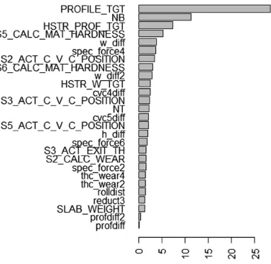
By observing the quality prediction model, the user can learn more about the quality property itself and how different process parameters affect it. The strength of the influence for each variable in the model correlates with the actual impact on the quality, and when the quality needs to be improved, the strongest variables are the first candidates to be considered. Figure4presents the relative influence of the variables in the profile deviation model. For example, process factors that relate to strength of the steel have a high impact on the profile deviation risk.

Fig. 4.The visualized variable importance in the GBM model for quality prediction.

(34)

deviation to both directions, whereas the large positive values of roll position (S2 ACT C V C POSITION) will increase the risk of negative profile deviation.

Fig. 5.The visualized effects of two variables in the GBM model for profile deviation prediction.

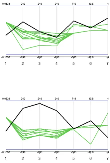
While analysing the prediction results of a product with a risk of a failure, the user typically asks what the difference between the observed one and good products is. Visually the difference can be effectively presented with parallel coordinates [18]. The comparison is not simple though, because, the determina-tion of a similar good products is a complex procedure. There is not only one way of making each product, but it is always a compromise forced by the status of the production line. Furthermore, there can be hundreds of different products with small modifications depending on the customer. In this application, the weight and height of a strip were used as similarity measures when fetching the best products from a pool of good products that can be used as examples of good production practices. Figure6presents two examples of products with negative predicted deviation from the profile target (black) and their comparison with similar good products (green). In the upper case, the observed product seems to have a bit higher value for parameters 2 and 7, but no clear candidates for quality improvement cannot be determined. In the lower case, variables 2, 3, 4 and 7 have a significant difference to the good products, and thus, the user will learn that those settings possess a higher risk for failure.

The comparison can be done also by calculating the distances between the curves. This way, a threshold can be set for showing high enough deviations from the good products. In Fig.7, the distances of an observed product are visually compared with the good ones. The customisation of the QMT has been made possible by offering several visualisation tool choices for the user.

4.2 Case 2: Strip Roughness

(35)

Fig. 6. The parallel coordinates visualize the difference between the good products (green) and the observed product (black) having an increased predicted risk for a failure. (Color figure online)

(36)

but also cold-rolling process parameters have a high impact on the surface. The QMT provides the user an easy to follow overall view to the process, and the user gets simple suggestions for improving the process, if an increased risk of defect occurred.

A typical user could be a process operator, who needs to concentrate on various information sources simultaneously. The presentation of the predicted quality have to be simple and it should support decision making when there is a limited time to react. The user would expect to have the following outputs that would assist him/her in decision making:

– colour-coded predicted quality during a selected time span for each product – clear visualization of recommended actions for a product with defect risk.

It is important that only relevant information is presented, or the user might start to neglect it. The chemical composition may have a high influence on the product quality, but at this point, the process operator have no possibility to modify it, and thus, the information is meaningless for the user. Instead, the process engineer is responsible for the improvement of the whole manufacturing process.

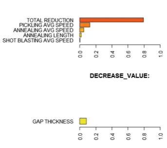
Figure8presents the information provided for the process operator, when the observed product has a risk of surface defect. It is easy to select which parameter should be adjusted, when no distracting information is present.

Fig. 8.Recommendations for process improvement.

5 Conclusion and Perspectives

(37)

Statistical quality models predict the quality of each product during the manufacturing, and the results are colour-coded to easily interpreted visual pre-sentations. When the user notices a deviant product or a period of defected products, it is easy to fetch more information about the product by selecting suitable actions. The provided visualizations will help to understand the model and factors that affect the prediction, and thus, the predicted quality as well. More advanced methods link the observed products with successful similar prod-ucts and highlight the differences in production. It can also recommend actions for quality improvement.

The QMT is having an online test period at both participating factories. The user feedback will provide us valuable information for further development of the tool. New user groups with different needs for information presentation will be included in the tool later. In its current version, the selected product can be compared with good ones fetched from a saved data set that has a large presentation of different product types. Later, the dynamicity will be improved by allowing the QMT to fetch an up to date comparison data from the online data base. As a result, it will be faster to find process settings that may be causing quality issues in constantly changing environment.

References

1. Harding, J., Shahbaz, M., Srinivas, Kusiak, A.: Data mining in manufacturing: a review. J. Manuf. Sci. Eng.128, 969–976 (2006)

2. Siirtola, P., Tamminen, S., Ferreira, E., Tiensuu, H., Prokkola, E., R¨oning, J.: Auto-matic recognition of steel plate side edge shape using classification and regression models. In: Proceedings of the 9th Eurosim Congress on Modelling and Simulation (EUROSIM 2016) (2016)

3. Phillips-Wren, G.: Intelligent decision support systems. In: Multicriteria Decision Aid and Artificial Intelligence. Wiley, Chichester (2013)

4. Logunova, O., Matsko, I., Posohov, I., Luk’ynov, S.: Automatic system for intel-ligent support of continuous cast billet production control processes. Int. J. Adv. Manuf. Technol.74, 1407–1418 (2014)

5. Dumitrache, I., Caramihai, S.: The intelligent manufacturing paradigm in knowl-edge society. In: Knowlknowl-edge Management. InTech, pp. 36–56 (2010)

6. Bi, Z., Xu, L., Wang, C.: Internet of things for enterprise systems of modern man-ufacturing. IEEE Trans. Ind. Inf.10(2), 1537–1546 (2014)

7. Xu, L., He, W., Li, S.: Internet of things in industries: a survey. IEEE Trans. Ind. Inf.10(4), 2233–2243 (2014)

8. Akram, M., Saif, A.W., Rahim, M.: Quality monitoring and process adjustment by integrating SPC and APC: a review. Int. J. Ind. Syst. Eng.11(4), 375–405 (2012) 9. Kano, M., Nakagawa, Y.: Data-based process monitoring, process control, and qual-ity improvement: recent developments and applications in steel industry. Comput. Chem. Eng.32(1–2), 12–24 (2008)

10. Bhadesia, H.: Neural networks in materials science. ISIJ Int. 39(10), 966–979 (1999)

(38)

12. Tamminen, S., Juutilainen, I., R¨oning, J.: Exceedance probability estimation for quality test consisting of multiple measurements. Expert Syst. Appl.40, 4577–4584 (2013)

13. Seni, G., Elder, J.: Ensemble methods in data mining: improving accuracy through combining predictions. In: Synthesis Lectures on Data Mining and Knowledge Dis-covery. Morgan & Claypool, USA (2010)

14. Natekin, A., Knoll, A.: Gradient boosting machines, a tutorial. Front. Neurorobot. 7(2013)

15. Elith, J., Leathwick, J., Hastie, T.: A working guide to boosted regression trees. J. Anim. Ecol.77, 802–813 (2008)

16. Friedman, J.: Stochastic gradient boosting. Comput. Stat. Data Anal.19, 367–378 (2002)

17. Juutilainen, I., Tamminen, S., R¨oning, J.: A tutorial to developing statistical mod-els for predictiong disqualification probability. In: Computational Methods for Optimizing Manufacturing Technology, Models and Techniques, pp. 368–399. IGI Global, USA (2012)

(39)

Mining Sequential Correlation

with a New Measure

Mohammad Fahim Arefin, Maliha Tashfia Islam, and Chowdhury Farhan Ahmed(B)

Department of Computer Science and Engineering, University of Dhaka, Dhaka, Bangladesh

[email protected], [email protected], [email protected]

Abstract. Being one of the most useful fields of data mining, sequential pattern mining is a very popular and much researched domain. However, simply pattern mining is often not enough to understand the intricate relationships that exist between data objects or items. A correlation mea-sure can uplift the task of mining interesting information that is useful to the end user. In this paper, we propose a new correlation measure, SequentialCorrelation, for sequential patterns. Along with that, we pro-pose a complete method calledSCM ineand design its efficient trie-based implementation. We use the measure to define a one or two way relation-ship between data objects and subsequently classify patterns into two subsets based on order dependency. Our performance study shows that a number of insignificant patterns can be pruned and it can give valuable insight into the datasets. SequentialCorrelation along with SCM ine can be very useful in many real life applications, especially because con-ventional correlation measures are not applicable in sequential datasets.

Keywords: Sequential pattern

·

Sequential correlation

Data mining

·

Sequential dependency

1 Introduction

Data mining is a field of science that deals with obtaining information (possibly unknown, interesting) from a huge amount of raw, unstructured data or repos-itories. One of the recently popular fields of data mining is sequential pattern mining. Sequential pattern mining [5] is quite similar to the classic data min-ing domain of frequent itemset minmin-ing. The main difference between the two is that, the order of items or data objects are not relevant in frequent itemset mining whereas sequential pattern mining specifically deals with data sequences where items are ordered. Sequential pattern mining methods are popularly used to identify patterns which are usually used in making recommendation systems, text predictions, improving system usability, making informative product choice decisions.

Many a times, even mining the frequent patterns or sequences are not enough. We would get a huge amount of patterns in lower support thresholds and only

c

Springer International Publishing AG, part of Springer Nature 2018 P. Perner (Ed.): ICDM 2018, LNAI 10933, pp. 29–43, 2018.

(40)

30 M. F. Arefin et al.

the obvious information from high thresholds. Correlation analysis is a useful tool here. Correlation analysis basically means finding out or measuring the strength of relationship among items, itemsets or data objects. The main moti-vation behind our work lies in the fact that there are not many widely known or standard correlation measures for sequential patterns.

For example, let’s suppose laptops and portable hard drives are frequently bought from a tech shop. Furthermore, there are 8 occurrences of Laptop =⇒ Hard Drive and 2 occurrences of Hard Drive =⇒ Laptop. In the total dataset there are 10 occurrences of each. In lower support thresholds, both these patterns are frequent but obviously we can decipher more about their relationship from the frequencies. There’s a 80% possibility that a laptop purchase will be followed by a purchase of hard drive, which means hard drives are generally bought after laptops.

Because we are working with sequential patterns, it is important that we retain information about the order in which they appeared while mining. If the sale of hard drives is found to be followed by the sale of laptop to a significant degree, this can be used in the real life application to boost sales or improve service. Otherwise if the order is not significant enough, advertising can be done in any form irrespective of order.

Our main contributions have been finding a null invariant correlation mea-sure for sequential patterns and constructing a complete method of using this measure, while keeping in mind the overhead for correlation analysis and per-formance benefits.

In the next section, some overview of previous works related to our field of application has been given. Section3contains the approach and algorithm with a short demonstration towards the end. Section4discusses the performance study and results obtained from it. Finally, we conclude with a small discussion about the future scope of our proposed methodology in Sect.5.

2 Related Work

(41)

Mining Sequential Correlation with a New Measure 31

works basically like PrefixSpan, the only addition being that a frequent sequence is only selected at each step if its prefix/suffix upperbound crosses a correlation threshold.

S2MP [10] is a similarity measure to compute the similarity of sequential patterns, which takes the characteristics and the semantics of sequential patterns into account. It considers the position of items as well as the number of common and non-common items in a sequence. A mapping score is given based on the resemblance of two sequences and an order score is given based the order and position of items in the sequences. Finally, S2MP is an aggregation of the two scores.

TheCMRules [3] is an association rule mining algorithm, which is based on the fact if we ignore or remove the time information of a sequence database, we obtain a transaction database. The algorithm ignores sequential information and mines the transaction database based on a minimum support and confidence threshold and generates the association rules. After that, sequential support and confidence of each rule is calculated by the sequential database and rules that do not meet the thresholds are eliminated. Since it uses general association rule mining, the execution time for CMRules grows proportionally to the number of association rules.

3 Our Proposed Approach

In this section, we will discuss:

– Our proposed measureSequentialCorrelation

– A complete algorithm for pattern categorization, SCM ine, along with its pseudo-code

– A suitable example for better understanding.

3.1 Terminologies

Itemset and Sequence: An itemset is denoted as (x1, x2, . . . , xk), wherexk is an item. Asequence is an ordered list of itemsets. A sequence S is denoted by s1s2, . . . , sl, where sj is an itemset or an element of the sequence.

Reverse Sequence: If a multi-itemset sequence is frequent, all of its sub pat-terns will be frequent also. So we consider each of the itemset to be atomic because an itemset is present in frequent pattern when the items in the itemset occur frequently, so it is significant as a whole.

So ifS=A(AB)CD, then reverse sequence of S,S′₌_DC(AB)A_.

(42)

32 M. F. Arefin et al.

sequential dataset then the sequence AB will be order dependent if the event, eA, containing A mostly comes before the event,eB, which contains B.

It is also denoted as a one way sequence becauseAB will be frequent in the dataset while BAfalls below the user defined support threshold i.e. the reverse sequence is infrequent.

Order Independent Sequences: An order independent sequence is defined as a sequence whose items have flexible order of appearance in the sequential database. For example, the sequenceABwill be order independent if the event, eA, containing A and the eventeB, which contains B have no dominant order. In other words, eA can occur before and aftereB in similar frequency in the total dataset.

SequentialCorrelation: Our measure,SequentialCorrelation, works by tak-ing the ratio of a certain pattern and its reverse with respect to their total occurrence. This gives us an estimate about the percentage or amount of pat-terns that follow a certain direction. We do not consider the total number of transactions because we wanted the measure to be null invariant.

Let F(A) be such a function that generates the frequency or total count of sequence A in the dataset. Here, A can be a sequence of itemsets. A’ will be the reverse sequence. For Example, ifA=A(AB)CD, thenA′₌_DC(AB)A_{. So} the Sequential Correlation becomes:

SequentialCorrelation, SC(A) =F(A)−F(A ′₎

F(A) +F(A′₎ (1)

The sequential correlation score will always have a value in the range [−1, 1] as all the itemsets in A will be frequent items or itemsets.|SC|= 0 will mean items are independent and |SC|= 1 will mean items have a very strong order dependency. A negative score represents that the reverse sequence is more significant. The score is also null-invariant as it doesn’t take null transactions into consideration.

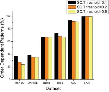
SequentialCorrelation Threshold (SC. Threshold): SequentialCorrelation Threshold denotes the tolerance or benchmark level for order dependency. Using a high threshold means that highly order dependent sequences are taken as interesting. A low threshold means that patterns or sequences can have flexibil-ity in ordering items. It is denoted as SC.T hreshold. Like support-confidence threshold, there is no universalSC.T hresholdvalue that is used. The threshold depends on the type of database, the data it carries and the particular objectives of the user.

3.2 Trie Architecture

(43)

Mining Sequential Correlation with a New Measure 33

memory usage because a lot of patterns or sequences will same the prefix or a partially similar prefix. It is essentially a tree with each node representing an element of the sequence. Each prefix is also stored only once.

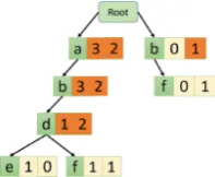
Suppose, the dataset contains the sequences{ABC:2, AD:3, BD:2}. The trie will have a root which contains links to the start of each sequence. The endpoint flags if the sequence upto that node is actually found in the dataset or it is just an intermediate node. The trie will look similar to Fig.1.

Fig. 1.Structure of the trie

3.3 Algorithm: SCM ine

Given a sequential database and the set of frequent sequences based on a user-defined support threshold, we need to find the sets of order dependent sequences and order independent sequences by usingSequentialCorrelationmeasure. The SC.T hresholdis also user-defined.

Step by Step Procedure: The prerequisite of our algorithm is a frequent pattern mining step. SCM ine assumes that any acceptable sequential pattern mining algorithm has been used to generate the list of frequent sequential pat-terns and their frequency count. Then the following steps are taken:

Advances in Data Mining. Applications and Theoretical Aspects

Petra Perner (Ed.)

123

LNAI 10933

18th Industrial Conference, ICDM 2018

New York, NY, USA, July 11–12, 2018

Proceedings

Advances in Data Mining

Lecture Notes in Arti

ﬁ

cial Intelligence

10933

Subseries of Lecture Notes in Computer Science

LNAI Series Editors

LNAI Founding Series Editor

Petra Perner (Ed.)

Advances in Data Mining

Applications and Theoretical Aspects

18th Industrial Conference, ICDM 2018

New York, NY, USA, July 11

–

12, 2018

Proceedings

Preface

Organization

Chair

Program Committee

Additional Reviewers

Contents

An Adaptive Oversampling Technique

for Imbalanced Datasets

·

·

·

1

Introduction

2

An Adaptive Oversampling Technique

3

Experiments

4

Conclusion

References

From Measurements to Knowledge

-Online Quality Monitoring and Smart

Manufacturing

·

·

·

·

1

Introduction

2

Developing a Quality Monitoring

Tool for Industrial Use

3

Statistical Quality Models

4

Quality Monitoring in Manufacturing

5

Conclusion and Perspectives

References

Mining Sequential Correlation

with a New Measure

·

·

1

Introduction

2

Related Work

3

Our Proposed Approach

_ﬁ

_–

_·

_·

_·

_·