Numerical Methods in Scientific Computing

(1)

(2)

Numerical

Methods

in Scientific

Computing

(3)

(4)

Numerical

Methods

in Scientific

Computing

Volume I

G

ERMUND

D

AHLQUIST

Royal Institute of Technology

Stockholm, Sweden

Å

KE

B

JÖRCK

Linköping University

Linköping, Sweden

(5)

10 9 8 7 6 5 4 3 2 1

All rights reserved. Printed in the United States of America. No part of this book may be reproduced, stored, or transmitted in any manner without the written permission of the publisher. For information, write to the Society for Industrial and Applied Mathematics, 3600 Market Street, 6th Floor, Philadelphia, PA 19104-2688 USA.

Trademarked names may be used in this book without the inclusion of a trademark symbol. These names are used in an editorial context only; no infringement of trademark is intended.

Mathematicais a registered trademark of Wolfram Research, Inc.

MATLAB is a registered trademark of The MathWorks, Inc. For MATLAB product information, please contact The MathWorks, Inc., 3 Apple Hill Drive, Natick, MA 01760-2098 USA, 508-647-7000, Fax: 508-647-7101, info@mathworks.com, www.mathworks.com.

Figure 4.5.2 originally appeared in Germund Dahlquist and Åke Björck. Numerical Methods. Prentice-Hall, 1974. It appears here courtesy of the authors.

Library of Congress Cataloging-in-Publication Data

Dahlquist, Germund.

Numerical methods in scientific computing / Germund Dahlquist, Åke Björck. p.cm.

Includes bibliographical references and index. ISBN 978-0-898716-44-3 (v. 1 : alk. paper)

1. Numerical analysis—Data processing. I. Björck, Åke, 1934- II. Title.

QA297.D335 2008

518—dc22 2007061806

(6)

To Marianne and Eva

(7)

(8)

Contents

List of Figures xv

List of Tables xix

List of Conventions xxi

Preface xxiii

1 Principles of Numerical Calculations 1

1.1 Common Ideas and Concepts . . . 1

1.1.1 Fixed-Point Iteration . . . 2

1.1.2 Newton’s Method . . . 5

1.1.3 Linearization and Extrapolation . . . 9

1.1.4 Finite Difference Approximations . . . 11

Review Questions . . . 15

Problems and Computer Exercises . . . 15

1.2 Some Numerical Algorithms . . . 16

1.2.1 Solving a Quadratic Equation . . . 16

1.2.2 Recurrence Relations . . . 17

1.2.3 Divide and Conquer Strategy . . . 20

1.2.4 Power Series Expansions . . . 22

1.3 Matrix Computations . . . 26

1.3.1 Matrix Multiplication . . . 26

1.3.2 Solving Linear Systems by LU Factorization . . . 28

1.3.3 Sparse Matrices and Iterative Methods . . . 38

1.3.4 Software for Matrix Computations . . . 41

1.4 The Linear Least Squares Problem . . . 44

1.4.1 Basic Concepts in Probability and Statistics . . . 45

1.4.2 Characterization of Least Squares Solutions . . . 46

1.4.3 The Singular Value Decomposition . . . 50

1.4.4 The Numerical Rank of a Matrix . . . 52

(9)

1.5 Numerical Solution of Differential Equations . . . 55

1.5.1 Euler’s Method . . . 55

1.5.2 An Introductory Example . . . 56

1.5.3 Second Order Accurate Methods . . . 59

1.5.4 Adaptive Choice of Step Size . . . 61

1.6 Monte Carlo Methods . . . 64

1.6.1 Origin of Monte Carlo Methods . . . 64

1.6.2 Generating and Testing Pseudorandom Numbers . . . 66

1.6.3 Random Deviates for Other Distributions . . . 73

1.6.4 Reduction of Variance . . . 77

Notes and References . . . 83

2 How to Obtain and Estimate Accuracy 87 2.1 Basic Concepts in Error Estimation . . . 87

2.1.1 Sources of Error . . . 87

2.1.2 Absolute and Relative Errors . . . 90

2.1.3 Rounding and Chopping . . . 91

2.2 Computer Number Systems . . . 93

2.2.1 The Position System . . . 93

2.2.2 Fixed- and Floating-Point Representation . . . 95

2.2.3 IEEE Floating-Point Standard . . . 99

2.2.4 Elementary Functions . . . 102

2.2.5 Multiple Precision Arithmetic . . . 104

2.3 Accuracy and Rounding Errors . . . 107

2.3.1 Floating-Point Arithmetic . . . 107

2.3.2 Basic Rounding Error Results . . . 113

2.3.3 Statistical Models for Rounding Errors . . . 116

2.3.4 Avoiding Overflow and Cancellation . . . 118

2.4 Error Propagation . . . 126

2.4.1 Numerical Problems, Methods, and Algorithms . . . 126

2.4.2 Propagation of Errors and Condition Numbers . . . 127

2.4.3 Perturbation Analysis for Linear Systems . . . 134

2.4.4 Error Analysis and Stability of Algorithms . . . 137

(10)

Contents ix

2.5 Automatic Control of Accuracy and Verified Computing . . . 145

2.5.1 Running Error Analysis . . . 145

2.5.2 Experimental Perturbations . . . 146

2.5.3 Interval Arithmetic . . . 147

2.5.4 Range of Functions . . . 150

2.5.5 Interval Matrix Computations . . . 153

3 Series, Operators, and Continued Fractions 157 3.1 Some Basic Facts about Series . . . 157

3.1.1 Introduction . . . 157

3.1.2 Taylor’s Formula and Power Series . . . 162

3.1.3 Analytic Continuation . . . 171

3.1.4 Manipulating Power Series . . . 173

3.1.5 Formal Power Series . . . 181

3.2 More about Series . . . 191

3.2.1 Laurent and Fourier Series . . . 191

3.2.2 The Cauchy–FFT Method . . . 193

3.2.3 Chebyshev Expansions . . . 198

3.2.4 Perturbation Expansions . . . 203

3.2.5 Ill-Conditioned Series . . . 206

3.2.6 Divergent or Semiconvergent Series . . . 212

3.3 Difference Operators and Operator Expansions . . . 220

3.3.1 Properties of Difference Operators . . . 220

3.3.2 The Calculus of Operators . . . 225

3.3.3 The Peano Theorem . . . 237

3.3.4 Approximation Formulas by Operator Methods . . . 242

3.3.5 Single Linear Difference Equations . . . 251

3.4 Acceleration of Convergence . . . 271

3.4.2 Comparison Series and Aitken Acceleration . . . 272

3.4.3 Euler’s Transformation . . . 278

3.4.4 Complete Monotonicity and Related Concepts . . . 284

3.4.5 Euler–Maclaurin’s Formula . . . 292

3.4.6 Repeated Richardson Extrapolation . . . 302

(11)

3.5 Continued Fractions and Padé Approximants . . . 321

3.5.1 Algebraic Continued Fractions . . . 321

3.5.2 Analytic Continued Fractions . . . 326

3.5.3 The Padé Table . . . 329

3.5.4 The Epsilon Algorithm . . . 336

3.5.5 The qd Algorithm . . . 339

4 Interpolation and Approximation 351 4.1 The Interpolation Problem . . . 351

4.1.2 Bases for Polynomial Interpolation . . . 352

4.1.3 Conditioning of Polynomial Interpolation . . . 355

4.2 Interpolation Formulas and Algorithms . . . 358

4.2.1 Newton’s Interpolation Formula . . . 358

4.2.2 Inverse Interpolation . . . 366

4.2.3 Barycentric Lagrange Interpolation . . . 367

4.2.4 Iterative Linear Interpolation . . . 371

4.2.5 Fast Algorithms for Vandermonde Systems . . . 373

4.2.6 The Runge Phenomenon . . . 377

4.3 Generalizations and Applications . . . 381

4.3.1 Hermite Interpolation . . . 381

4.3.2 Complex Analysis in Polynomial Interpolation . . . 385

4.3.3 Rational Interpolation . . . 389

4.3.4 Multidimensional Interpolation . . . 395

4.3.5 Analysis of a Generalized Runge Phenomenon . . . 398

4.4 Piecewise Polynomial Interpolation . . . 410

4.4.1 Bernštein Polynomials and Bézier Curves . . . 411

4.4.2 Spline Functions . . . 417

4.4.3 The B-Spline Basis . . . 426

4.4.4 Least Squares Splines Approximation . . . 434

4.5 Approximation and Function Spaces . . . 439

4.5.1 Distance and Norm . . . 440

4.5.2 Operator Norms and the Distance Formula . . . 444

(12)

Contents xi

4.5.4 Solution of the Approximation Problem . . . 454

4.5.5 Mathematical Properties of Orthogonal Polynomials . . . 457

4.5.6 Expansions in Orthogonal Polynomials . . . 466

4.5.7 Approximation in the Maximum Norm . . . 471

4.6 Fourier Methods . . . 482

4.6.1 Basic Formulas and Theorems . . . 483

4.6.2 Discrete Fourier Analysis . . . 487

4.6.3 Periodic Continuation of a Function . . . 491

4.6.4 Convergence Acceleration of Fourier Series . . . 492

4.6.5 The Fourier Integral Theorem . . . 494

4.6.6 Sampled Data and Aliasing . . . 497

4.7 The Fast Fourier Transform . . . 503

4.7.1 The FFT Algorithm . . . 503

4.7.2 Discrete Convolution by FFT . . . 509

4.7.3 FFTs of Real Data . . . 510

4.7.4 Fast Trigonometric Transforms . . . 512

4.7.5 The General Case FFT . . . 515

5 Numerical Integration 521 5.1 Interpolatory Quadrature Rules . . . 521

5.1.2 Treating Singularities . . . 525

5.1.3 Some Classical Formulas . . . 527

5.1.4 Superconvergence of the Trapezoidal Rule . . . 531

5.1.5 Higher-Order Newton–Cotes’ Formulas . . . 533

5.1.6 Fejér and Clenshaw–Curtis Rules . . . 538

5.2 Integration by Extrapolation . . . 546

5.2.1 The Euler–Maclaurin Formula . . . 546

5.2.2 Romberg’s Method . . . 548

5.2.3 Oscillating Integrands . . . 554

5.2.4 Adaptive Quadrature . . . 560

5.3 Quadrature Rules with Free Nodes . . . 565

5.3.1 Method of Undetermined Coefficients . . . 565

(13)

5.3.3 Gauss Quadrature with Preassigned Nodes . . . 573

5.3.4 Matrices, Moments, and Gauss Quadrature . . . 576

5.3.5 Jacobi Matrices and Gauss Quadrature . . . 580

5.4 Multidimensional Integration . . . 587

5.4.1 Analytic Techniques . . . 588

5.4.2 Repeated One-Dimensional Integration . . . 589

5.4.3 Product Rules . . . 590

5.4.4 Irregular Triangular Grids . . . 594

5.4.5 Monte Carlo Methods . . . 599

5.4.6 Quasi–Monte Carlo and Lattice Methods . . . 601

6 Solving Scalar Nonlinear Equations 609 6.1 Some Basic Concepts and Methods . . . 609

6.1.2 The Bisection Method . . . 610

6.1.3 Limiting Accuracy and Termination Criteria . . . 614

6.1.4 Fixed-Point Iteration . . . 618

6.1.5 Convergence Order and Efficiency . . . 621

6.2 Methods Based on Interpolation . . . 626

6.2.1 Method of False Position . . . 626

6.2.2 The Secant Method . . . 628

6.2.3 Higher-Order Interpolation Methods . . . 631

6.2.4 A Robust Hybrid Method . . . 634

6.3 Methods Using Derivatives . . . 637

6.3.1 Newton’s Method . . . 637

6.3.2 Newton’s Method for Complex Roots . . . 644

6.3.3 An Interval Newton Method . . . 646

6.3.4 Higher-Order Methods . . . 647

6.4 Finding a Minimum of a Function . . . 656

6.4.2 Unimodal Functions and Golden Section Search . . . 657

6.4.3 Minimization by Interpolation . . . 660

(14)

Contents xiii

6.5 Algebraic Equations . . . 662

6.5.1 Some Elementary Results . . . 662

6.5.2 Ill-Conditioned Algebraic Equations . . . 665

6.5.3 Three Classical Methods . . . 668

6.5.4 Deflation and Simultaneous Determination of Roots . . . 671

6.5.5 A Modified Newton Method . . . 675

6.5.6 Sturm Sequences . . . 677

6.5.7 Finding Greatest Common Divisors . . . 680

Bibliography 687

Index 707

A Online Appendix: Introduction to Matrix Computations A-1

A.1 Vectors and Matrices . . . A-1 A.1.1 Linear Vector Spaces . . . A-1 A.1.2 Matrix and Vector Algebra . . . A-3 A.1.3 Rank and Linear Systems . . . A-5 A.1.4 Special Matrices . . . A-6 A.2 Submatrices and Block Matrices . . . A-8 A.2.1 Block Gaussian Elimination . . . A-10 A.3 Permutations and Determinants . . . A-12 A.4 Eigenvalues and Norms of Matrices . . . A-16 A.4.1 The Characteristic Equation . . . A-16 A.4.2 The Schur and Jordan Normal Forms . . . A-17 A.4.3 Norms of Vectors and Matrices . . . A-18 Review Questions . . . A-21 Problems . . . A-22

B Online Appendix: A MATLAB Multiple Precision Package B-1

(15)

C Online Appendix: Guide to Literature C-1

(16)

List of Figures

1.1.1 Geometric interpretation of iterationxn₊1=F (xn). . . 3

1.1.2 The fixed-point iterationxn₊1=(xn+c/xn)/2,c=2,x0=0.75. . . . 4

1.1.3 Geometric interpretation of Newton’s method. . . 7

1.1.4 Geometric interpretation of the secant method. . . 8

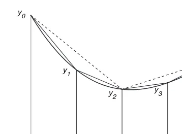
1.1.5 Numerical integration by the trapezoidal rule(n₌4). . . 10

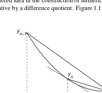
1.1.6 Centered finite difference quotient. . . 11

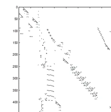
1.3.1 Nonzero pattern of a sparse matrix from an eight stage chemical distilla-tion column. . . 39

1.3.2 Nonzero structure of the matrixA(left) andL₊U(right). . . 39

1.3.3 Structure of the matrixA(left) andL₊U(right) for the Poisson problem, N ₌20 (rowwise ordering of the unknowns). . . 41

1.4.1 Geometric characterization of the least squares solution. . . 48

1.4.2 Singular values of a numerically singular matrix. . . 53

1.5.1 Approximate solution of the differential equationdy/dt ₌y,y0=0.25, by Euler’s method withh₌0.5. . . 56

1.5.2 Approximate trajectories computed with Euler’s method withh₌0.01. 58 1.6.1 Neutron scattering. . . 66

1.6.2 Plots of pairs of 106_{random uniform deviates}_(U i, Ui₊1)such thatUi < 0.0001. Left: MATLAB 4; Right: MATLAB 5. . . 71

1.6.3 Random number with distributionF (x). . . 74

1.6.4 Simulated two-dimensional Brownian motion. Plotted are 32 simulated paths withh₌0.1, each consisting of 64 steps. . . 76

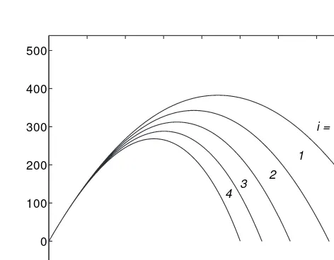
1.6.5 The left part shows how the estimate of π varies with the number of throws. The right part compares_|m/n₋2/π_|with the standard deviation ofm/n. . . 78

1.6.6 Mean waiting times for doctor and patients at polyclinic. . . 81

2.2.1 Positive normalized numbers whenβ ₌2,t ₌3, and₋1_≤e_≤2. . . 97

2.2.2 Positive normalized and denormalized numbers whenβ₌2,t ₌3, and −1≤e_≤2. . . 99

2.3.1 Computed values forn ₌ 10p, p ₌ 1 _: 14, of_|(1₊1/n)n₋e_|and |exp(nlog(1₊1/n))₋e_|. . . 110

2.3.2 Calculated values of a polynomial near a multiple root. . . 117

2.3.3 The frequency function of the normal distribution forσ ₌1. . . 118

(17)

2.4.1 Geometrical illustration of the condition number. . . 134

2.5.1 Wrapping effect in interval analysis. . . 152

3.1.1 Comparison of a series with an integral,(n₌5). . . 160

3.1.2 A series whereRnandRn+1have different signs. . . 161

3.1.3 Successive sums of an alternating series. . . 161

3.1.4 Partial sums of the Maclaurin expansions for two functions. The upper curves are for cosx,n₌0_:2_:26, 0_≤x _≤10. The lower curves are for 1/(1₊x2),n₌0_:2_:18, 0_≤x _≤1.5. . . 163

3.1.5 Relative error in approximations of the error function by a Maclaurin series truncated after the first term that satisfies the condition in (3.1.11). 165 3.2.1 Graph of the Chebyshev polynomialT20(x),x∈ [−1,1]. . . 200

3.2.2 Example 3.2.7(A): Terms of (3.2.33), cn = (n+1)−2, x = 40, no preconditioner. . . 208

3.2.3 Example 3.2.7(B):cn=(n+1)−2,x=40, with preconditioner in(3.2.36). . . 209

3.2.4 Error estimates of the semiconvergent series of Example 3.2.9 forx ₌10; see(3.2.43). . . 213

3.2.5 The error of the expansion off (x)₌1/(1₊x2)in a sum of Chebyshev polynomials{Tn(x/1.5)},n≤12. . . 216

3.3.1 Bounds for truncation error RT and roundoff errorRXF in numerical differentiation as functions ofh(U ₌0.5_·10−6). . . 248

3.4.1 Logarithms of the actual errors and the error estimates for MN,k in a more extensive computation for the alternating series in (3.4.12)with completely monotonic terms. The tolerance is here set above the level where the irregular errors become important; for a smaller tolerance parts of the lowest curves may become less smooth in some parts. . . 283

3.5.1 Best rational approximations_{(p, q)_}to the “golden ratio.” . . . 325

4.2.1 Error of interpolation inPnforf (x)=xn, usingn=12: Chebyshev points (solid line) and equidistant points (dashed line). . . 378

4.2.2 Polynomial interpolation of 1/(1₊25x2)in two ways using 11 points: equidistant points (dashed curve), Chebyshev abscissae (dashed-dotted curve). . . 378

(18)

List of Figures xvii

4.3.3 log₁₀_|(f₋Lnf )(u)|for Runge’s classical examplef (u)=1/(1+25u2)

with 30equidistant nodes in _[−1,1_]. The oscillating curves are the

empirical interpolation errors (observed at 300 equidistant points), for

u₌xin the lower curve and foru₌x₊0.02iin the upper curve; in both

casesx_{∈ [−}1,1_]. The smooth curves are the estimates of these quantities

obtained by the logarithmic potential model; see Examples 4.3.10 and

4.3.11. . . 403

4.3.4 Some level curves of the logarithmic potential associated with Chebyshev interpolation. They are ellipses with foci at±1. Due to the symmetry only a quarter is shown of each curve. The value ofℜψ (z)for a curve is seen to the left, close to the curve. . . 404

4.4.1 The four cubic Bernštein polynomials. . . 412

4.4.2 Quadratic Bézier curve with control points. . . 414

4.4.3 Cubic Bézier curve with control pointsp0, . . . , p3. . . 414

4.4.4 De Casteljau’s algorithm forn₌2,t ₌ 1₂. . . 416

4.4.5 A drafting spline. . . 417

4.4.6 Broken line and cubic spline interpolation. . . 419

4.4.7 Boundary slope errorseB,ifor a cubic spline,e0=em = −1;m=20. . 426

4.4.8 Formation of a double knot for a linear spline. . . 428

4.4.9 B-splines of orderk₌1,2,3. . . 429

4.4.10 The four cubic B-splines nonzero forx_∈(t₀, t₁)with coalescing exterior knotst₋3=t−2 =t−1=t0. . . 430

4.4.11 Banded structure of the matricesAandAT_A_{arising in cubic spline} ap-proximation with B-splines (nonzero elements shown). . . 435

4.4.12 Least squares cubic spline approximation of titanium data using 17 knots marked on the axes by an “o.” . . . 436

4.5.1 The Legendre polynomialP21. . . 463

4.5.2 Magnitude of coefficientsci in a Chebyshev expansion of an analytic function contaminated with roundoff noise. . . 472

4.5.3 Linear uniform approximation. . . 475

4.6.1 A rectangular wave. . . 486

4.6.2 Illustration of Gibbs’ phenomenon. . . 487

4.6.3 Periodic continuation of a functionf outside_[0, π_]as an odd function. 491 4.6.4 The real (top) and imaginary (bottom) parts of the Fourier transform (solid line) ofe−xand the corresponding DFT (dots) withN₌32,T ₌8. . . 499

5.1.1 The coefficients_|am,j|of theδ2-expansion form=2 :2 :14,j =0 : 20. The circles are the coefficients for the closed Cotes’ formulas, i.e., j ₌1₊m/2. . . 537

5.2.1 The Filon-trapezoidal rule applied to the Fourier integral withf (x)₌ex_, forh₌1/10, andω₌1_:1000; solid line: exact integral; dashed line: absolute value of the error. . . 558

5.2.2 The oscillating functionx−1cos(x−1lnx). . . 559

5.2.3 A needle-shaped function. . . 561

5.4.1 RegionDof integration. . . 590

(19)

5.4.3 Refinement of a triangular grid. . . 594

5.4.4 Barycentric coordinates of a triangle. . . 595

5.4.5 Correction for curved boundary segment. . . 598

5.4.6 The grids forI4andI16. . . 599

5.4.7 Hammersley points in[0,1_]2. . . 603

6.1.1 Graph of curvesy ₌(x/2)2and sinx. . . 611

6.1.2 The bisection method. . . 612

6.1.3 Limited-precision approximation of a continuous function. . . 615

6.1.4 The fixed-point iterationxk₊1=e−xk,_x 0 =0.3. . . 619

6.2.1 The false-position method. . . 627

6.2.2 The secant method. . . 628

6.3.1 The functionx₌ulnu. . . 642

6.3.2 A situation where Newton’s method converges from anyx0∈ [a, b]. . . 643

6.4.1 One step of interval reduction,g(ck)≥g(dk). . . 658

(20)

List of Tables

1.6.1 Simulation of waiting times for patients at a polyclinic. . . 80

2.2.1 IEEE floating-point formats. . . 100

2.2.2 IEEE 754 representation. . . 101

2.4.1 Condition numbers of Hilbert matrices of order_≤12. . . 135

3.1.1 Maclaurin expansions for some elementary functions. . . 167

3.2.1 Results of three ways to compute F (x)₌(1/x)₀x(1/t )(1₋e−t_{) dt}_{. . . .} ₂₀₇

3.2.2 Evaluation of some Bessel functions. . . 211

3.3.1 Bickley’s table of relations between difference operators. . . 231

3.3.2 Integratingy′′ _{= −}y,y(0)₌ 0,y′(0) ₌ 1; the letters U and S in the headings of the last two columns refer to “Unstable” and “Stable.” . . . 258

3.4.1 Summation by repeated averaging. . . 278

3.4.2 Bernoulli and Euler numbers;B1= −1/2, E1=1. . . 294

4.5.1 Weight functions and recurrence coefficients for some classical monic orthogonal polynomials. . . 465

4.6.1 Useful symmetry properties of the continuous Fourier transform. . . 495

4.7.1 Useful symmetry properties of the DFT. . . 511

5.1.1 The coefficientswi =Aciin then-point closed Newton–Cotes’ formulas. 534 5.1.2 The coefficientswi =Aciin then-point open Newton–Cotes’ formulas. 535 5.3.1 Abscissae and weight factors for some Gauss–Legendre quadrature from [1, Table 25.4]. . . 572

6.5.1 The qd scheme for computing the zeros ofLy(z). . . 674

6.5.2 Left: Sign variations in the Sturm sequence. Right: Intervals[lk, uk] containing the zeroxk. . . 679

(21)

(22)

List of Conventions

Besides the generally accepted mathematical abbreviations and notations (see, e.g., James and James,Mathematics Dictionary[1985, pp. 467–471]), the following notations are used in the book:

MATLAB_{has been used for this book in testing algorithms. We also use its notations}

for array operations and the convenient colon notation.

._∗ A ._∗Belement-by-element productA(i, j )B(i, j )

./ A ./Belement-by-element divisionA(i, j )/B(i, j )

i_:k same asi, i₊1, . . . , kand empty ifi > k i_:j _:k same asi, i₊j, i₊2j, . . . , k

A(_:, k), A(i,_:) thekth column,ith row ofA, respectively A(i_:k) same asA(i), A(i₊1), . . . , A(k)

⌊x_⌋ floor, i.e., the largest integer_≤x

⌈x_⌉ roof, i.e., the smallest integer_≥x exand exp(x) both denote the exponential function

fl(x₊y) floating-point operations; see Sec. 2.2.3

{xi}ni=0 denotes the set{x0, x1, . . . , xn}

[a, b_] closed interval(a_≤x _≤b)

(a, b) open interval(a < x < b)

sign(x) ₊1 ifx _≥0, else₋1

int(a, b, c, . . . , w) the smallest interval which containsa, b, c, . . . , w f (x)₌O(g(x)),x _→a _|f (x)/g(x)_|is bounded asx_→a

(acan be finite,_+∞, or_−∞) f (x)₌o(g(x)),x _→a limx→af (x)/g(x)=0

f (x)_∼g(x),x _→a limx→af (x)/g(x)=1

k_≤i, j_≤n meansk_≤i_≤nandk_≤j _≤n

Pk the set of polynomials of degreeless thank

(f, g) scalar product of functionsf andg

· p p-norm in a linear vector or function space;

see Sec. 4.5.1–4.5.3 and Sec. A.3.3 in Online Appendix A

En(f ) dist(f,Pn)∞,[a,b]; see Definition 4.5.6

The notationsa _≈ b, a b, and a b are defined in Sec. 2.1.2. Matrices and

vectors are generally denoted by Roman lettersAandb. AT _and_bT _{denote the transpose}

of the matrixAand the vectorb, respectively. (A, B)means a partitioned matrix; see Sec.

A.2 in Online Appendix A. Notation for matrix computation can also be found in Online Appendix A. Notations for differences and difference operators, e.g.,42yn,[x0, x1, x2]f,

δ2y, are defined in Chapters 3 and 4.

(23)

(24)

Preface

In 1974 the book by Dahlquist and Björck, Numerical Methods, was published in the Prentice–Hall Series in Automatic Computation, edited by George Forsythe. It was an extended and updated English translation of a Swedish undergraduate textbook used at the Royal Institute of Technology (KTH) in Stockholm. This book became one of the most successful titles at Prentice–Hall. It was translated into several other languages and as late as 1990 a Chinese edition appeared. It was reprinted in 2003 by Dover Publications.

In 1984 the authors were invited by Prentice–Hall to prepare a new edition of the book. After some attempts it soon became apparent that, because of the rapid development of the field, one volume would no longer suffice to cover the topics treated in the 1974 book. Thus a large part of the new book would have to be written more or less from scratch. This meant more work than we initially envisaged. Other commitments inevitably interfered, sometimes for years, and the project was delayed. The present volume is the result of several revisions worked out during the past 10 years.

Tragically, my mentor, friend, and coauthor Germund Dahlquist died on February 8, 2005, before this first volume was finished. Fortunately the gaps left in his parts of the manuscript were relatively few. Encouraged by his family, I decided to carry on and I have tried to the best of my ability to fill in the missing parts. I hope that I have managed to convey some of his originality and enthusiasm for his subject. It was a great privilege for me to work with him over many years. It is sad that he could never enjoy the fruits of his labor on this book.

Today mathematics is used in one form or another within most areas of science and industry. Although there has always been a close interaction between mathematics on the one hand and science and technology on the other, there has been a tremendous increase in the use of sophisticated mathematical models in the last decades. Advanced mathematical models and methods are now also used more and more within areas such as medicine, economics, and social sciences. Today, experiment and theory, the two classical elements of the scientific method, are supplemented in many areas by computations that are an equally important component.

The increased use of numerical methods has been caused not only by the continuing advent of faster and larger computers. Gains in problem-solving capabilities through bet-ter mathematical algorithms have played an equally important role. In modern scientific computing one can now treat more complex and less simplified problems through massive amounts of numerical calculations.

This volume is suitable for use in a basic introductory course in a graduate program in numerical analysis. Although short introductions to numerical linear algebra and differential

(25)

equations are included, a more substantial treatment is deferred to later volumes. The book can also be used as a reference for researchers in applied sciences working in scientific computing. Much of the material in the book is derived from graduate courses given by the first author at KTH and Stanford University, and by the second author at Linköping University, mainly during the 1980s and 90s.

We have aimed to make the book as self-contained as possible. The level of presenta-tion ranges from elementary in the first and second chapters to fairly sophisticated in some later parts. For most parts the necessary prerequisites are calculus and linear algebra. For some of the more advanced sections some knowledge of complex analysis and functional analysis is helpful, although all concepts used are explained.

The choice of topics inevitably reflects our own interests. We have included many methods that are important in large-scale computing and the design of algorithms. But the emphasis is on traditional and well-developed topics in numerical analysis. Obvious omissions in the book are wavelets and radial basis functions. Our experience from the 1974 book showed us that the most up-to-date topics are the first to become out of date.

Chapter 1 is on a more elementary level than the rest of the book. It is used to introduce a few general and powerful concepts and ideas that will be used repeatedly. An introduction is given to some basic methods in the numerical solution of linear equations and least squares problems, including the important singular value decomposition. Basic techniques for the numerical solution of initial value problems for ordinary differential equations is illustrated. An introduction to Monte Carlo methods, including a survey of pseudorandom number generators and variance reduction techniques, ends this chapter.

Chapter 2 treats floating-point number systems and estimation and control of errors. It is modeled after the same chapter in the 1974 book, but the IEEE floating-point standard has made possible a much more satisfactory treatment. We are aware of the fact that this aspect of computing is considered by many to be boring. But when things go wrong (and they do!), then some understanding of floating-point arithmetic and condition numbers may be essential. A new feature is a section on interval arithmetic, a topic which recently has seen a revival, partly because the directed rounding incorporated in the IEEE standard simplifies the efficient implementation.

In Chapter 3 different uses of infinite power series for numerical computations are studied, including ill-conditioned and semiconvergent series. Various algorithms for com-puting the coefficients of power series are given. Formal power series are introduced and their convenient manipulation using triangular Toeplitz matrices is described.

Difference operators are handy tools for the derivation, analysis, and practical ap-plication of numerical methods for many tasks such as interpolation, differentiation, and quadrature. A more rigorous treatment of operator series expansions and the use of the Cauchy formula and the fast Fourier transform (FFT) to derive the expansions are original features of this part of Chapter 3.

(26)

Preface xxv

An exposition of continued fractions and Padé approximation, which transform a (formal) power series into a sequence of rational functions, concludes this chapter. This includes theǫ-algorithm, the most important nonlinear convergence acceleration method,

as well as the qd algorithm.

Chapter 4 treats several topics related to interpolation and approximation. Different bases for polynomial interpolation and related interpolation formulas are explained. The advantages of the barycentric form of Lagrange interpolation formula are stressed. Complex analysis is used to derive a general Lagrange–Hermite formula for polynomial interpolation in the complex plane. Algorithms for rational and multidimensional interpolation are briefly surveyed.

Interpolation of an analytic function at an infinite equidistant point set is treated from the point of view of complex analysis. Applications made to the Runge phenomenon and the Shannon sampling theorem. This section is more advanced than the rest of the chapter and can be skipped in a first reading.

Piecewise polynomials have become ubiquitous in computer aided design and com-puter aided manufacturing. We describe how parametric Bézier curves are constructed from piecewise Bernštein polynomials. A comprehensive treatment of splines is given and the famous recurrence relation of de Boor and Cox for B-splines is derived. The use of B-splines for representing curves and surfaces with given differentiability conditions is illustrated.

Function spaces are introduced in Chapter 4 and the concepts of linear operator and operator norm are extended to general infinite-dimensional vector spaces. The norm and distance formula, which gives a convenient error bound for general approximation problems, is presented. Inner product spaces, orthogonal systems, and the least squares approximation problem are treated next. The importance of the three-term recurrence formula and the Stieltjes procedure for numerical calculations is stressed. Chebyshev systems and theory and algorithms for approximation in maximum norm are surveyed.

Basic formulas and theorems for Fourier series and Fourier transforms are discussed next. Periodic continuation, sampled data and aliasing, and the Gibbs phenomenon are treated. In applications such as digital signal and image processing, and time-series analysis, the FFT algorithm (already used in Chapter 3) is an important tool. A separate section is therefore devoted to a matrix-oriented treatment of the FFT, including fast trigonometric transforms.

In Chapter 5 the classical Newton–Cotes rules for equidistant nodes and the Clenshaw– Curtis interpolatory rules for numerical integration are first treated. Next, extrapolation methods such as Romberg’s method and the use of the ǫ-algorithm are described. The

superconvergence of the trapezoidal rule in special cases and special Filon-type methods for oscillating integrands are discussed. A short section on adaptive quadrature follows.

Quadrature rules with both free and prescribed nodes are important in many contexts. A general technique of deriving formulas using the method of undetermined coefficients is given first. Next, Gauss–Christoffel quadrature rules and their properties are treated, and Gauss–Lobatto, Gauss–Radau, and Gauss–Kronrod rules are introduced. A more advanced exposition of relations between moments, tridiagonal matrices, and Gauss quadrature is included, but this part can be skipped at first reading.

(27)

interpolation formulas on such grids are derived. Together with a simple correction for curved boundaries these formulas are also very suitable for use in the finite element method. A discussion of Monte Carlo and quasi–Monte Carlo methods and their advantages for high-dimensional integration ends Chapter 5.

Chapter 6 starts with the bisection method. Next, fixed-point iterations are introduced and the contraction mapping theorem proved. Convergence order and the efficiency index are discussed. Newton’s method is treated also for complex-valued equations and an interval Newton method is described. A discussion of higher-order methods, including the Schröder family of methods, is featured in this chapter.

Because of their importance for the matrix eigenproblem, algebraic equations are treated at length. The frequent ill-conditioning of roots is illustrated. Several classical methods are described, as well as an efficient and robust modified Newton method due to Madsen and Reid. Further, we describe the progressive qd algorithm and Sturm sequence methods, both of which are also of interest for the tridiagonal eigenproblem.

Three Online Appendices are available from the Web page of the book,www.siam. org/books/ot103. Appendix A is a compact survey of notations and some frequently used results in numerical linear algebra. Volume II will contain a full treatment of these topics. Online Appendix B describes Mulprec, a collection of MATLAB m-files for (almost) unlimited high precision calculation. This package can also be downloaded from the Web page. Online Appendix C is a more complete guide to literature, where advice is given on not only general textbooks in numerical analysis but also handbooks, encyclopedias, tables, software, and journals.

An important feature of the book is the large collection of problems and computer exercises included. This draws from the authors’ 40+ year of experience in teaching courses in numerical analysis. It is highly recommended that a modern interactive system such as MATLAB is available to the reader for working out these assignments. The 1974 book also contained answers and solutions to most problems. It has not been possible to retain this feature because of the much greater number and complexity of the problems in the present book.

We have aimed to make and the bibliography as comprehensive and up-to-date as possible. A Notes and References section containing historical comments and additional references concludes each chapter. To remind the reader of the fact that much of the the-ory and many methods date one or several hundred years back in time, we have included more than 60 short biographical notes on mathematicians who have made significant con-tributions. These notes would not have been possible without the invaluable use of the bi-ographies compiled at the School of Mathematics and Statistics, University of St Andrews, Scotland (www-history.mcs.st.andrews.ac.uk). Many of these full biographies are fascinating to read.

(28)

Preface xxvii

Per Lötstedt. Thank you all for your interest in the book and for giving so much of your valuable time!

The book was typeset in LA_{TEX the references were prepared in BibTEX, and the index} with MakeIndex. These are all wonderful tools and my thanks goes to Donald Knuth for his gift to mathematics. Thanks also to Cleve Moler for MATLAB, which was used in working out examples and for generating figures.

It is a pleasure to thank Elizabeth Greenspan, Sarah Murphy, and other staff at SIAM for their cheerful and professional support during all phases of the acquisition and production of the book.

Åke Björck

(29)

(30)

Chapter 1

Principles of Numerical

Calculations

It is almost impossible to identify a mathematical theory no matter how “pure,” that has never influenced numerical reasoning.

—B. J. C. Baxter and Arieh Iserles

1.1 Common Ideas and Concepts

Although numerical mathematics has been used for centuries in one form or another within many areas of science and industry,1_{modern scientific computing using electronic} comput-ers has its origin in research and developments during the Second World War. In the late 1940s and early 1950s the foundation of numerical analysis was laid as a separate discipline of mathematics. The new capability of performing billions of arithmetic operations cheaply has led to new classes of algorithms, which need careful analysis to ensure their accuracy and stability.

As a rule, applications lead to mathematical problems which in their complete form cannot be conveniently solved with exact formulas, unless one restricts oneself to special cases or simplified models. In many cases, one thereby reduces the problem to a sequence of linear problems—for example, linear systems of differential equations. Such an approach can quite often lead to concepts and points of view which, at least qualitatively, can be used even in the unreduced problems.

Recent developments have enormously increased the scope for using numerical meth-ods. Gains in problem solving capabilities mean that today one can treat much more complex and less simplified problems through massive amounts of numerical calculations. This has increased the interaction of mathematics with science and technology.

In most numerical methods, one applies a small number of general and relatively simple ideas. These are then combined with one another in an inventive way and with such

1_{The Greek mathematician Archimedes (287–212 B.C.), Isaac Newton (1642–1727), and Carl Friedrich Gauss} (1777–1883) were pioneering contributors to numerical mathematics.

(31)

knowledge of the given problem as one can obtain in other ways—for example, with the methods of mathematical analysis. Some knowledge of the background of the problem is also of value; among other things, one should take into account the orders of magnitude of certain numerical data of the problem.

In this chapter we shall illustrate the use of some general ideas behind numerical methods on some simple problems. These may occur as subproblems or computational details of larger problems, though as a rule they more often occur in a less pure form and on a larger scale than they do here. When we present and analyze numerical methods, to some degree we use the same approach which was first mentioned above: we study in detail special cases and simplified situations, with the aim of uncovering more generally applicable concepts and points of view which can guide us in more difficult problems.

It is important to keep in mind that the success of the methods presented depends on the smoothness properties of the functions involved. In this first survey we shall tacitly assume that the functions have as many well-behaved derivatives as are needed.

1.1.1 Fixed-Point Iteration

One of the most frequently occurring ideas in numerical calculations is iteration(from

the Latiniterare, “to plow once again”) orsuccessive approximation. Taken generally, iteration means the repetition of a pattern of action or process. Iteration in this sense occurs, for example, in the repeated application of a numerical process—perhaps very complicated and itself containing many instances of the use of iteration in the somewhat narrower sense to be described below—in order to improve previous results. To illustrate a more specific use of the idea of iteration, we consider the problem of solving a (usually) nonlinear equation of the form

x₌F (x), (1.1.1)

whereF is assumed to be a differentiable function whose value can be computed for any

given value of a real variablex, within a certain interval. Using the method of iteration,

one starts with an initial approximationx0, and computes the sequence

x1=F (x0), x2=F (x1), x3=F (x2), . . . . (1.1.2) Each computation of the type xn₊1 = F (xn), n = 0,1,2, . . . , is called a fixed-point

iteration. Asngrows, we would like the numbersxnto be better and better estimates of

the desired root. If the sequence_{xn}converges to a limiting valueα, then we have

α₌ lim

n→∞xn+1=nlim→∞F (xn)=F (α),

and thusx₌αsatisfies the equationx₌F (x). One can then stop the iterations when the

desired accuracy has been attained.

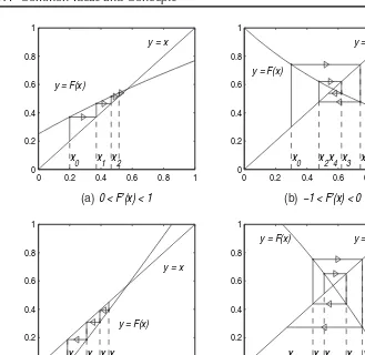
A geometric interpretation of fixed point iteration is shown in Figure 1.1.1. A root of (1.1.1) is given by the abscissa (and ordinate) of an intersecting point of the curvey ₌F (x)

and the liney₌x. Starting fromx0, the pointx1=F (x0)on thex-axis is obtained by first drawing a horizontal line from the point(x0, F (x0)) =(x0, x1)until it intersects the line

(32)

1.1. Common Ideas and Concepts 3

0 0.2 0.4 0.6 0.8 1

0 0.2 0.4 0.6 0.8 1 x

0 x1 x2

0 < F′(x) < 1 y = F(x)

y = x

0 0.2 0.4 0.6 0.8 1

0 0.2 0.4 0.6 0.8 1 x

0 x2x4x3 x1

−1 < F′(x) < 0 y = F(x)

y = x

0 0.2 0.4 0.6 0.8 1

0 0.2 0.4 0.6 0.8 1 x 0 x 1 x 2 x 3

F′(x) > 1 y = F(x)

y = x

0 0.2 0.4 0.6 0.8 1

0 0.2 0.4 0.6 0.8 1 x

0 x1

x

2 x3

x

4

F′(x) < −1

y = F(x) y = x

(a) (b)

(c) (d)

Figure 1.1.1. Geometric interpretation of iterationxn+1=F (xn).

and so on in a “staircase” pattern. In Figure 1.1.1(a) it is obvious that the sequence{xn}

converges monotonically to the rootα. Figure 1.1.1(b) shows a case whereFis a decreasing

function. There we also have convergence, but not monotone convergence; the successive iteratesxnlie alternately to the right and to the left of the rootα. In this case the root is

bracketed by any two successive iterates.

There are also two divergent cases, exemplified by Figures 1.1.1(c) and (d). One can see geometrically that the quantity, which determines the rate of convergence (or diver-gence), is the slope of the curvey ₌F (x)in the neighborhood of the root. Indeed, from

the mean value theorem of calculus we have

xn₊1−α

xn−α =

F (xn)−F (α)

xn−α =

F′(ξn),

whereξnlies betweenxnandα. We see that ifx0 is chosen sufficiently close to the root (yetx0=α), the iteration will converge if|F′(α)|<1. In this caseαis called apoint of

attraction. The convergence is faster the smaller_|F′(α)_|is. If_|F′(α)_| > 1, thenαis a

(33)

0.5 1 1.5 2 2.5 0.5

1 1.5 2 2.5

x₀ x₂ x₁

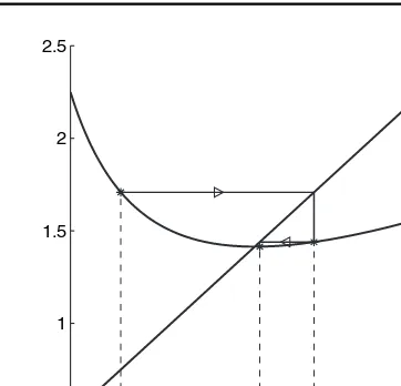
Figure 1.1.2. The fixed-point iterationxn+1=(xn+c/xn)/2,c=2,x0 =0.75.

Example 1.1.1.

The square root of c >0 satisfies the equationx2 ₌ c, which can also be written x₌c/xorx ₌(x₊c/x)12. This suggests the fixed-point iteration

xn₊1= 1₂(xn+c/xn) , n=1,2, . . . , (1.1.3)

which is the widely usedHeron’s rule.2 The curvey ₌F (x)is in this case a hyperbola

(see Figure 1.1.2).

From (1.1.3) follows

xn+1±√c= 1 2

xn±2

√

c₊ c xn

= (xn± √

c)2

2xn ;

that is,

xn₊1−√c

xn+1+√c =

xn−√c

xn+√c

2

. (1.1.4)

We can takeen= xn−

√_c

xn+√c to be a measure of the error inxn. Then (1.1.4) readsen+1 =e

2

n

and it follows thaten=e2

n

0 . If|x0−√c| = |x0+√c|, thene0 <1 andxnconverges to a

square root ofcwhenn_{→ ∞}. Note that the iteration (1.1.3) can also be used for complex

values ofc.

Forc₌2 andx0 =1.5, we getx1 =(1.5+2/1.5)12=15/12=1.4166666. . . , and

x2=1.414215 686274, x3=1.414213 562375

(34)

rapid convergence is due to the fact that forα₌√cwe have F′(α)₌(1₋c/α2)/2₌0.

One can in fact show that

lim

n→∞

|xn+1−√c|

|xn−√c|2 =

C

for some constant 0 < C < _∞, which is an example of what is known as quadratic convergence. Roughly, ifxnhastcorrect digits, thenxn+1will have at least 2t−1 correct digits.

The above iteration method is used quite generally on both pocket calculators and larger computers for calculating square roots.

Iteration is one of the most important aids for practical as well as theoretical treatment of both linear and nonlinear problems. One very common application of iteration is to the solution ofsystems of equations. In this case{xn}is a sequence of vectors, andF is a

vector-valued function. When iteration is applied todifferential equations,{xn}means a sequence

of functions, andF (x)means an expression in which integration or other operations on

functions may be involved. A number of other variations on the very general idea of iteration will be given in later chapters.

The form of (1.1.1) is frequently called thefixed-point form, since the rootαis a

fixed point of the mappingF. An equation may not be given in this form originally. One

has a certain amount of choice in the rewriting of an equationf (x) ₌ 0 in fixed-point

form, and the rate of convergence depends very much on this choice. The equationx2₌c

can also be written, for example, asx ₌c/x. The iteration formulaxn+1 =c/xngives a

sequence which alternates betweenx0(for evenn) andc/x0(for oddn)—the sequence does not converge for anyx₀₌√c!

1.1.2 Newton’s Method

Let an equation be given in the formf (x)₌0, and for anyk₌0, set F (x)₌x₊kf (x).

Then the equation x ₌ F (x) is equivalent to the equationf (x) ₌ 0. Since F′(α) ₌

1₊kf′(α), we obtain the fastest convergence fork_{= −}1/f′(α). Becauseαis not known,

this cannot be applied literally. But if we usexnas an approximation, this leads to the choice

F (x)₌x₋f (x)/f′_(x)_{, or the iteration}

xn+1=xn−

f (xn)

f′_(x_n₎. (1.1.5)

(35)

The equationx2₌ccan be written in the formf (x)₌x2₋c₌0. Newton’s method

for this equation becomes

xn₊1=xn−

x_n2₋c

2xn =

1 2

xn+

c xn

, n₌0,1,2, . . . , (1.1.6)

which is the fast method in Example 1.1.1. More generally, Newton’s method applied to the equationf (x)₌xp₋_c₌_{0 can be used to compute}_c1/p_,_p_{= ±}₁_,_±₂_{, . . . ,}_{from the}

iteration

xn₊1=xn−

xnp−c

pxnp−1

.

This can be written as

xn₊1= 1

p

(p₋1)xn+

c

xpn−1

= xn

(₋p)[(1−p)−cx

−p

n ]. (1.1.7)

It is convenient to use the first expression in (1.1.7) whenp > 0 and the second when p <0. Withp ₌2,3, and₋2, respectively, this iteration formula is used for calculating

√_c,√3_c_{, and 1}_/√_c_{. Also 1}_/c_{, (}_p

= −1) can be computed by the iteration

xn+1=xn+xn(1−cxn)=xn(2−cxn),

using only multiplication and addition. In some early computers, which lacked division in hardware, this iteration was used to implement division, i.e.,b/cwas computed asb(1/c).

Example 1.1.2.

We want to construct an algorithm based on Newton’s method for the efficient calcu-lation of the square root of any given floating-point numbera. If we first shift the mantissa

so that the exponent becomes even,a₌c_·22e_{, and 1}_/₂_≤_{c <}_{2; then}

√

a ₌√c_·2e.

We need only consider the reduced range 1/2_≤c_≤1 since for 1< c_≤2 we can compute

√₁

/cand invert.4

To find an initial approximationx0to start the Newton iterations when 1/2≤c <1, we can use linear interpolation ofx ₌√cbetween the endpoints 1/2,1, giving

x0(c)=√2(1−c)+2(c−1/2) (√2 is precomputed). The iteration then proceeds using (1.1.6).

Forc₌3/4 (√c₌0.86602540378444) the result isx0 =(√2+2)/4 and (correct digits are in boldface)

x0=0.85355339059327, x1 =0.86611652351682,

x₂ ₌0.86602540857756, x₃ ₌0.86602540378444,

(36)

The quadratic rate of convergence is apparent. Three iterations suffice to give about 16 digits of accuracy for allx_{∈ [}1/2,1_].

Newton’s method is based onlinearization. This means thatlocally, i.e., in a small

neighborhood of a point,a more complicated function is approximated with a linear func-tion. In the solution of the equationf (x) ₌0, this means geometrically that we seek the

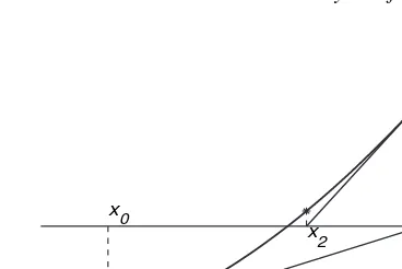
intersection point between thex-axis and the curvey ₌f (x); see Figure 1.1.3. Assume

x₀

x₁ x₂

Figure 1.1.3. Geometric interpretation of Newton’s method.

that we have an approximating valuex₀to the root. We then approximate the curve with its tangentat the point(x0, f (x0)). Letx1be the abscissa of the point of intersection between thex-axis and the tangent. Since the equation for the tangent reads

y₋f (x0)=f′(x0)(x−x0), by settingy ₌0 we obtain the approximation

x1=x0−f (x0)/f′(x0).

In many casesx1 will have about twice as many correct digits asx0. But ifx0is a poor approximation andf (x)far from linear, then it is possible thatx1will be a worse approxi-mation thanx0.

If we combine the ideas of iteration and linearization, that is, substitutexnforx0and

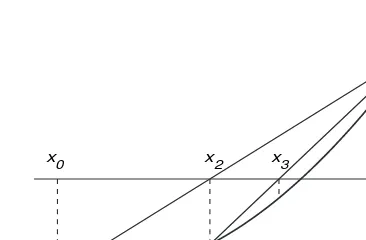
xn+1forx1, we rediscover Newton’s method mentioned earlier. Ifx0is close enough toα, the iterations will converge rapidly (see Figure 1.1.3), but there are also cases of divergence. An alternative to drawing the tangent to approximate a curve locally with a linear function is to choose two neighboring points on the curve and to approximate the curve with thesecantwhich joins the two points; see Figure 1.1.4. Thesecant methodfor the

solution of nonlinear equations is based on this approximation. This method, which preceded Newton’s method, is discussed in more detail in Sec. 6.3.1.

Newton’s method can be generalized to yield a quadratically convergent method for solving asystem of nonlinear equations

(37)

x

1

x

0 x2 x3

Figure 1.1.4. Geometric interpretation of the secant method.

Such systems arise in many different contexts in scientific computing. Important examples are the solution of systems of differential equations and optimization problems. We can write (1.1.8) asf(x)₌0, wherefandxare vectors inRn_{. The vector-valued function}_f _is

said to be differentiable at the pointxif each component is differentiable with respect to all

the variables. The matrix of partial derivatives offwith respect tox,

J (x)₌f′(x)₌   

∂f1 ∂x1 . . .

∂f1 ∂xn ..

. ...

∂fn

∂x1 . . . ∂fn

∂xn  

∈Rn×n, (1.1.9)

is called theJacobianoff.

Letxkbe the current approximate solution and assume that the matrixf′(xk)is

nonsin-gular. Then inNewton’s methodfor the system (1.1.8), the next iteratexn₊1is determined from the unique solution to the system of linear equations

J (xk)(xn₊1−xk)= −f(xk). (1.1.10)

The linear system (1.1.10) can be solved by computing the LU factorization of the matrix

J (x); see Sec. 1.3.2.

Each step of Newton’s method requires the evaluation of then2entries of the Jacobian

matrixJ (xk). This may be a time consuming task ifn is large. If either the iterates or

the Jacobian matrix are not changing too rapidly, it is possible to reevaluateJ (xk)only

occasionally and use the same Jacobian in several steps. This has the further advantage that once we have computed the LU factorization of the Jacobian matrix, the linear system can be solved in onlyO(n2)arithmetic operations; see Sec. 1.3.2.

Example 1.1.3.

The following example illustrates the quadratic convergence of Newton’s method for simple roots. The nonlinear system

(38)

has a solution close tox0=0.5,y0=1. The Jacobian matrix is

J (x, y)₌

2x₋4 2y

2 2y

,

and Newton’s method becomes

xk+1

yk+1

=

xk

yk

−J (xk, yk)−1

x_k2₊y_k2₋4xn

y_k2₊2xk−2

.

We get the following results:

k xk yk

1 0.35 1.15

2 0.35424528301887 1.13652584085316

3 0.35424868893322 1.13644297217273

4 0.35424868893541 1.13644296914943

All digits are correct in the last iteration. The quadratic convergence is obvious; the number of correct digits approximately doubles in each iteration.

Often, the main difficulty in solving a nonlinear system is to find a sufficiently good starting point for the Newton iterations. Techniques for modifying Newton’s method to ensure global convergenceare therefore important in several dimensions. These must

include techniques for coping with ill-conditioned or even singular Jacobian matrices at intermediate points. Such techniques will be discussed in Volume II.

1.1.3 Linearization and Extrapolation

The secant approximation is useful in many other contexts; for instance, it is generally used when one “reads between the lines” or interpolates in a table of numerical values. In this case the secant approximation is calledlinear interpolation. When the secant approximation is used innumerical integration, i.e., in the approximate calculation of a definite integral,

I ₌

b

a

y(x) dx, (1.1.11)

(see Figure 1.1.5) it is called thetrapezoidal rule. With this method, the area between the

curvey ₌y(x)and thex-axis is approximated with the sumT (h)of the areas of a series

of parallel trapezoids. Using the notation of Figure 1.1.5, we have

T (h)₌h1

2

n₋1

i=0

(yi+yi₊1), h=

b₋a

n . (1.1.12)

(In the figure, n ₌ 4.) We shall show in a later chapter that the error is very nearly

proportional to h2 when h is small. One can then, in principle, attain arbitrarily high

(39)

a b

y₀

y

1

y

2

y₃

y₄

Figure 1.1.5. Numerical integration by the trapezoidal rule(n₌4).

proportional to the number of points wherey(x)must be computed, and thus inversely

proportional toh. Hence the computational work grows rapidly as one demands higher

accuracy (smallerh).

Numerical integration is a fairly common problem because only seldom can the “prim-itive” function be analytically calculated in a finite expression containing only elementary functions. It is not possible for such simple functions asex2_or₍_sin_x)/x_{. In order to obtain}

higher accuracywith significantly less work than the trapezoidal rule requires, one can use one of the following two important ideas:

(a) local approximationof the integrand with a polynomial of higher degree, or with a

function of some other class, for which one knows the primitive function;

(b) computation with the trapezoidal rule for several values ofhand then extrapolation

toh ₌ 0, the so-calledRichardson extrapolation5 or deferred approach to the limit, with the use of general results concerning the dependence of the error onh.

The technical details for the various ways of approximating a function with a poly-nomial, including Taylor expansions, interpolation, and the method of least squares, are treated in later chapters.

The extrapolation to the limit can easily be applied to numerical integration with the trapezoidal rule. As was mentioned previously, the trapezoidal approximation (1.1.12) to the integral has an error approximately proportional to the square of the step size. Thus, using two step sizes,hand 2h, one has

T (h)₋I _≈kh2, T (2h)₋I _≈k(2h)2,

and hence 4(T (h)₋I )_≈T (2h)₋I, from which it follows that I _≈ 1

3(4T (h)−T (2h))=T (h)+ 1

3(T (h)−T (2h)).

(40)

Thus, by adding the corrective term1

3(T (h)−T (2h))toT (h), one should get an estimate of I which is typically far more accurate thanT (h). In Sec. 3.4.6 we shall see that the

improvement is in most cases quite striking. The result of the Richardson extrapolation is in this case equivalent to the classicalSimpson’s rulefor numerical integration, which

we shall encounter many times in this volume. It can be derived in several different ways. Section 3.4.5 also contains application of extrapolation to problems other than numerical integration, as well as a further development of the extrapolation idea, namelyrepeated Richardson extrapolation. In numerical integration this is also known as Romberg’s method; see Sec. 5.2.2.

Knowledge of the behavior of the error can, together with the idea of extrapolation, lead to a powerful method for improving results. Such a line of reasoning is useful not only for the common problem of numerical integration, but also in many other types of problems.

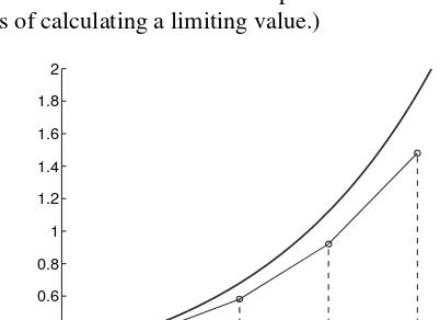
Example 1.1.4.

The integral

12

10

f (x) dx

is computed forf (x)₌x3by the trapezoidal method. Withh₌1 we obtainT (h)₌2695, T (2h)₌2728, and extrapolation givesT ₌2684, equal to the exact result.

Similarly, forf (x) ₌ x4 we obtain T (h) ₌ 30,009, T (2h) ₌ 30,736, and with

extrapolationT _≈29,766.7 (exact 29,766.4).

1.1.4 Finite Difference Approximations

The local approximation of a complicated function by a linear function leads to another frequently encountered idea in the construction of numerical methods, namely the approx-imation of a derivative by a difference quotient. Figure 1.1.6 shows the graph of a function

(n − 1)h nh (n + 1)h y_n₋₁

y_n

y_n+1

(41)

y(x)in the interval_[xn−1, xn+1], wherexn+1−xn =xn−xn−1 =h;his called the step size. If we setyi =y(xi),i=n−1, n, n+1, then the derivative atxncan be approximated

by aforward differencequotient,

y′(xn)≈

yn+1−yn

h , (1.1.13)

or a similar backward difference quotient involvingynandyn−1. The error in the approxi-mation is called adiscretization error.

But it is conceivable that thecentered differenceapproximation

y′(xn)≈

yn+1−yn−1

2h (1.1.14)

usually will be more accurate. It is in fact easy to motivate this. By Taylor’s formula,

y(x₊h)₋y(x)₌y′(x)h₊y′′(x)h2/2₊y′′′(x)h3/6_{+ · · ·}, (1.1.15)

−y(x₋h)₊y(x)₌y′(x)h₋y′′(x)h2/2₊y′′′(x)h3/6_{− · · ·}. (1.1.16)

Setx₌xn. Then, by the first of these equations,

y′(xn)=

yn+1−yn

h −

h

2y′′(xn)− · · ·.

Next, add the two Taylor expansions and divide by 2h. Then the first error term cancels and

we have

y′(xn)=

yn₊1−yn₋1 2h −

h2

6 y′′′(xn)− · · ·. (1.1.17)

In what follows we call a formula (or a method), where a step size parameterhis involved,

accurate of orderp, if its error is approximately proportional tohp. Sincey′′(x)vanishes

for allxif and only ifyis a linear function ofx, and similarly,y′′′(x)vanishes for allx if

and only ifyis a quadratic function, we have established the following important result.

Lemma 1.1.1.

The forward difference approximation(1.1.13)is exact only for a linear function, and it is only first order accurate in the general case. The centered difference approximation (1.1.14)is exact also for a quadratic function, and is second order accurate in the general case.

For the above reason the approximation(1.1.14)is, in most situations, preferable

(42)

Higher derivatives can be approximated withhigher differences, that is, differences

of differences, another central concept in numerical calculations. We define

(4y)n=yn+1−yn;

(42y)n=(4(4y))n=(yn₊2−yn₊1)−(yn₊1−yn)

=yn+2−2yn+1+yn;

(43y)n=(4(42y))n=yn+3−3yn+2+3yn+1−yn;

etc. For simplicity one often omits the parentheses and writes, for example,42y5 instead of(42y)₅. The coefficients that appear here in the expressions for the higher differences

are, by the way, the binomial coefficients. In addition, if we denote the step length by4x

instead of byh, we get the following formulas, which are easily remembered:

dy

dx ≈

4y 4x,

d2y dx2 ≈

42y

(4x)2, (1.1.18)

etc. Each of these approximations is second order accurate for the value of the derivative at anxwhich equals themean valueof the largest and smallestxfor which the corresponding

value ofy is used in the computation of the difference. (The formulas are only first order

accurate when regarded as approximations to derivatives at other points between these bounds.) These statements can be established by arguments similar to the motivation for (1.1.13) and (1.1.14).

Taking the difference of the Taylor expansions (1.1.15)–(1.1.16) with one more term in each and dividing byh2, we obtain the following important formula:

y′′(xn)=

yn₊1−2yn+yn₋1

h2 −

h2

12y

iv_(x

n)− · · ·.

Introducing thecentral difference operator

δyn=y

xn+

1 2h

−y

xn−

1 2h

(1.1.19)

and neglecting higher order terms we get

y′′(xn)≈

1

h2δ

2_y

n−

h2

12y

iv_(x

n). (1.1.20)

The approximation of (1.1.14) can be interpreted as an application of (1.1.18) with

4x ₌2h, or as the mean of the estimates which one gets according to (1.1.18) fory′((n₊

1

2)h)andy′((n−12)h).

When the values of the function have errors (for example, when they are rounded numbers) the difference quotients become more and more uncertain the smallerhis. Thus

if one wishes to compute the derivatives of a function one should be careful not to use too small a step length; see Sec. 3.3.4.

Example 1.1.5.

Assume that fory ₌cosx, function values correct to six decimal digits are known at

(43)

x y 4y 42y

0.59 0.830941

−5605

0.60 0.825336 ₋83

−5688

0.61 0.819648

,

where the differences are expressed in units of 10−6_{. This arrangement of the numbers is} called adifference scheme. Using (1.1.14) and (1.1.18) one gets

y′(0.60)_≈(0.819648₋0.830941)/0.02_{= −}0.56465, y′′(0.60)_{≈ −}83_·10−6/(0.01)2_{= −}0.83.

The correct results are, with six decimals,

y′(0.60)_{= −}0.564642, y′′(0.60)_{= −}0.825336.

In y′′ we got only two correct decimal digits. This is due tocancellation, which is an

important cause of loss of accuracy; see Sec. 2.3.4. Better accuracy can be achieved by

increasingthe steph; see Problem 1.1.5 at the end of this section.

A very important equation of mathematical physics isPoisson’s equation:6

∂2u ∂x2 +

∂2u

∂y2 =f (x, y), (x, y)∈<. (1.1.21)

Here the function f (x, y) is given together with some boundary condition onu(x, y).

Under certain conditions, gravitational, electric, magnetic, and velocity potentials satisfy

Laplace’s equation7 which is (1.1.21) withf (x, y)₌0.

Finite difference approximations are useful for partial derivatives. Suppose that<is

a rectangular region and introduce arectangular gridthat covers the rectangle. With grid

spacinghandk, respectively, in thex andy directions, respectively, this consists of the

points

xi=x0+ih, i=0:M, yj =y0+j k, j =0:N.

By (1.1.20), a second order accurate approximation of Poisson’s equation is given by the

five-point operator

∇52u=

ui₊1,j −2ui,j +ui₋1,j

h2 +

ui,j₊1−2ui,j+ui,j₋1

k2 .

Fork₌h

∇52u= 1

h2

ui,j+1+ui−1,j −4ui,j +ui+1,j+ui,j−1,

6_{Siméon Denis Poisson (1781–1840), professor at École Polytechnique. He has also given his name t}