IPython Interactive
Computing and
Visualization
Cookbook
Over 100 hands-on recipes to sharpen your skills in
high-performance numerical computing and data
science with Python
Cyrille Rossant
IPython Interactive Computing and
Visualization Cookbook
Copyright © 2014 Packt Publishing
All rights reserved. No part of this book may be reproduced, stored in a retrieval system, or transmitted in any form or by any means, without the prior written permission of the publisher, except in the case of brief quotations embedded in critical articles or reviews.
Every effort has been made in the preparation of this book to ensure the accuracy of the information presented. However, the information contained in this book is sold without warranty, either express or implied. Neither the author, nor Packt Publishing, and its dealers and distributors will be held liable for any damages caused or alleged to be caused directly or indirectly by this book.
Packt Publishing has endeavored to provide trademark information about all of the companies and products mentioned in this book by the appropriate use of capitals. However, Packt Publishing cannot guarantee the accuracy of this information.
First published: September 2014
Production reference: 1190914
Published by Packt Publishing Ltd. Livery Place
35 Livery Street
Birmingham B3 2PB, UK.
ISBN 978-1-78328-481-8
About the Author
Cyrille Rossant
is a researcher in neuroinformatics, and is a graduate of Ecole Normale Supérieure, Paris, where he studied mathematics and computer science. He has worked at Princeton University, University College London, and Collège de France.As part of his data science and software engineering projects, he gained experience in machine learning, high-performance computing, parallel computing, and big data visualization. He is one of the developers of Vispy, a high-performance visualization
package in Python. He is the author of Learning IPython for Interactive Computing and Data Visualization, Packt Publishing, a beginner-level introduction to data analysis in Python, and the prequel of this book.
I would like to thank the IPython development team for their support. I am also deeply grateful to Nick Fiorentini and his partner Darbie Whitman for their invaluable help during the later stages of editing.
About the Reviewers
Chetan Giridhar
is an open source evangelist and Python enthusiast. He has been invited to talk at international Python conferences on topics such as filesystems, search engines, and real-time communication. He is also working as an associate editor at Python editorial, The Python Papers Anthology.Chetan works as a lead engineer and evangelist at BlueJeans Network
(http://bluejeans.com/), a leading video conferencing site on Cloud Company.
He has co-authored an e-book, Design Patterns in Python, Testing Perspective, and has reviewed books on Python programming at Packt Publishing.
I'd like to thank my parents (Jayant and Jyotsana Giridhar), my wife Deepti, and my friends/colleagues for supporting and inspiring me.
Robert Johansson
has a PhD in Theoretical Physics from Chalmers University of Technology, Sweden. He is currently working as a researcher at the Interdisciplinary Theoretical Science Research Group at RIKEN, Japan, focusing on computational condensed-matter physics and quantum mechanics.Jose Unpingco
is the author of the Python for Signal Processing blog and thecorresponding book. A graduate from University of California, San Diego, he has spent almost 20 years in the industry as an analyst, instructor, engineer, consultant, and technical director in the area of signal processing. His interests include time-series analysis, statistical signal processing, random processes, and large-scale interactive computing.
www.PacktPub.com
Support files, eBooks, discount offers, and more
You might want to visit www.PacktPub.com for support files and downloads related to your book.
Did you know that Packt offers eBook versions of every book published, with PDF and ePub files available? You can upgrade to the eBook version at www.PacktPub.com and as a print book customer, you are entitled to a discount on the eBook copy. Get in touch with us at [email protected] for more details.
At www.PacktPub.com, you can also read a collection of free technical articles, sign up for a range of free newsletters and receive exclusive discounts and offers on Packt books and eBooks.
TM
http://PacktLib.PacktPub.com
Do you need instant solutions to your IT questions? PacktLib is Packt's online digital book library. Here, you can access, read and search across Packt's entire library of books.
Why Subscribe?
f Fully searchable across every book published by Packt f Copy and paste, print and bookmark content
f On demand and accessible via web browser
Free Access for Packt account holders
Table of Contents
Preface 1
Chapter 1: A Tour of Interactive Computing with IPython
9
Introduction 9
Introducing the IPython notebook 13
Getting started with exploratory data analysis in IPython 22 Introducing the multidimensional array in NumPy for fast array computations 28 Creating an IPython extension with custom magic commands 32 Mastering IPython's configuration system 36
Creating a simple kernel for IPython 39
Chapter 2: Best Practices in Interactive Computing
45
Introduction 45 Choosing (or not) between Python 2 and Python 3 46 Efficient interactive computing workflows with IPython 50 Learning the basics of the distributed version control system Git 53 A typical workflow with Git branching 56 Ten tips for conducting reproducible interactive computing experiments 59
Writing high-quality Python code 63
Writing unit tests with nose 67
Debugging your code with IPython 74
Chapter 3: Mastering the Notebook
79
Introduction 79
Table of Contents
Creating a custom JavaScript widget in the notebook – a spreadsheet
editor for pandas 103
Processing webcam images in real time from the notebook 108
Chapter 4: Profiling and Optimization
115
Introduction 115 Evaluating the time taken by a statement in IPython 116 Profiling your code easily with cProfile and IPython 117 Profiling your code line-by-line with line_profiler 121 Profiling the memory usage of your code with memory_profiler 124 Understanding the internals of NumPy to avoid unnecessary array copying 127
Using stride tricks with NumPy 133
Implementing an efficient rolling average algorithm with stride tricks 135 Making efficient array selections in NumPy 138 Processing huge NumPy arrays with memory mapping 140 Manipulating large arrays with HDF5 and PyTables 142 Manipulating large heterogeneous tables with HDF5 and PyTables 146
Chapter 5: High-performance Computing
149
Introduction 149 Accelerating pure Python code with Numba and Just-In-Time compilation 154 Accelerating array computations with Numexpr 158 Wrapping a C library in Python with ctypes 159 Accelerating Python code with Cython 163 Optimizing Cython code by writing less Python and more C 167 Releasing the GIL to take advantage of multi-core processors
with Cython and OpenMP 174
Writing massively parallel code for NVIDIA graphics cards (GPUs)
with CUDA 175
Writing massively parallel code for heterogeneous platforms
with OpenCL 181
Distributing Python code across multiple cores with IPython 185 Interacting with asynchronous parallel tasks in IPython 189 Parallelizing code with MPI in IPython 192 Trying the Julia language in the notebook 195
Chapter 6: Advanced Visualization
201
Introduction 201
Table of Contents
Getting started with Vispy for high-performance interactive
data visualizations 218
Chapter 7: Statistical Data Analysis
225
Introduction 225 Exploring a dataset with pandas and matplotlib 229 Getting started with statistical hypothesis testing – a simple z-test 233 Getting started with Bayesian methods 236 Estimating the correlation between two variables with a contingency
table and a chi-squared test 241
Fitting a probability distribution to data with the maximum
likelihood method 245
Estimating a probability distribution nonparametrically with
a kernel density estimation 251
Fitting a Bayesian model by sampling from a posterior distribution
with a Markov chain Monte Carlo method 255 Analyzing data with the R programming language in the
IPython notebook 261
Chapter 8: Machine Learning
267
Introduction 267
Getting started with scikit-learn 273
Predicting who will survive on the Titanic with logistic regression 281 Learning to recognize handwritten digits with a K-nearest
neighbors classifier 285
Learning from text – Naive Bayes for Natural Language Processing 289 Using support vector machines for classification tasks 293 Using a random forest to select important features for regression 298 Reducing the dimensionality of a dataset with a principal
component analysis 302
Detecting hidden structures in a dataset with clustering 306
Chapter 9: Numerical Optimization
311
Introduction 311 Finding the root of a mathematical function 314
Minimizing a mathematical function 317
Fitting a function to data with nonlinear least squares 323 Finding the equilibrium state of a physical system by minimizing
its potential energy 326
Chapter 10: Signal Processing
333
Introduction 333 Analyzing the frequency components of a signal with
Table of Contents
Applying a linear filter to a digital signal 343 Computing the autocorrelation of a time series 349
Chapter 11: Image and Audio Processing
353
Introduction 353 Manipulating the exposure of an image 355
Applying filters on an image 358
Segmenting an image 362
Finding points of interest in an image 367 Detecting faces in an image with OpenCV 370 Applying digital filters to speech sounds 373 Creating a sound synthesizer in the notebook 377
Chapter 12: Deterministic Dynamical Systems
381
Introduction 381 Plotting the bifurcation diagram of a chaotic dynamical system 383 Simulating an elementary cellular automaton 387 Simulating an ordinary differential equation with SciPy 390 Simulating a partial differential equation – reaction-diffusion systems
and Turing patterns 394
Chapter 13: Stochastic Dynamical Systems
401
Introduction 401
Simulating a discrete-time Markov chain 402
Simulating a Poisson process 406
Simulating a Brownian motion 410
Simulating a stochastic differential equation 412
Chapter 14: Graphs, Geometry, and Geographic
Information Systems
417
Introduction 417
Manipulating and visualizing graphs with NetworkX 421 Analyzing a social network with NetworkX 425 Resolving dependencies in a directed acyclic graph with
a topological sort 430
Computing connected components in an image 434 Computing the Voronoi diagram of a set of points 438 Manipulating geospatial data with Shapely and basemap 442 Creating a route planner for a road network 446
Chapter 15: Symbolic and Numerical Mathematics
453
Table of Contents
Analyzing real-valued functions 458
Computing exact probabilities and manipulating random variables 460
A bit of number theory with SymPy 462
Finding a Boolean propositional formula from a truth table 465 Analyzing a nonlinear differential system – Lotka-Volterra
(predator-prey) equations 467
Getting started with Sage 470
Preface
We are becoming awash in the flood of digital data from scientific research, engineering, economics, politics, journalism, business, and many other domains. As a result, analyzing, visualizing, and harnessing data is the occupation of an increasingly large and diverse set of people. Quantitative skills such as programming, numerical computing, mathematics, statistics, and data mining, which form the core of data science, are more and more appreciated in a seemingly endless plethora of fields.
My previous book, Learning IPython for Interactive Computing and Data Visualization, Packt Publishing, published in 2013, was a beginner-level introduction to data science and numerical computing with Python. This widely-used programming language is also one of the most popular platforms for these disciplines.
This book continues that journey by presenting more than 100 advanced recipes for data science and mathematical modeling. These recipes not only cover programming and computing topics such as interactive computing, numerical computing, high-performance computing, parallel computing, and interactive visualization, but also data analysis topics such as statistics, data mining, machine learning, signal processing, and many others.
Preface
What this book is
This cookbook contains in excess of a hundred focused recipes, answering specific questions in numerical computing and data analysis with IPython on:
f How to explore a public dataset with pandas, PyMC, and SciPy
f How to create interactive plots, widgets, and Graphical User Interfaces in the IPython notebook
f How to create a configurable IPython extension with custom magic commands
f How to distribute asynchronous tasks in parallel with IPython
f How to accelerate code with OpenMP, MPI, Numba, Cython, OpenCL, CUDA, and the Julia programming language
f How to estimate a probability density from a dataset
f How to get started using the R statistical programming language in the notebook f How to train a classifier or a regressor with scikit-learn
f How to find interesting projections in a high-dimensional dataset
f How to detect faces in an image
f How to simulate a reaction-diffusion system f How to compute an itinerary in a road network
The choice made in this book was to introduce a wide range of different topics instead of delving into the details of a few methods. The goal is to give you a taste of the incredibly rich capabilities of Python for data science. All methods are applied on diverse real-world examples.
Every recipe of this book demonstrates not only how to apply a method, but also how and why it works. It is important to understand the mathematical concepts and ideas underlying the methods instead of merely applying them blindly.
Additionally, each recipe comes with many references for the interested reader who wants to know more. As online references change frequently, they will be kept up to date on the book's website (http://ipython-books.github.io).
What this book covers
This book is split into two parts:Part 1 (chapters 1 to 6) covers advanced methods in interactive numerical computing, high-performance computing, and data visualization.
Preface
Part 1 – Advanced High-Performance Interactive
Computing
Chapter 1, A Tour of Interactive Computing with IPython, contains a brief but intense introduction to data analysis and numerical computing with IPython. It not only covers common packages such as Python, NumPy, pandas, and matplotlib, but also advanced IPython topics such as interactive widgets in the notebook, custom magic commands, configurable IPython extensions, and new language kernels.
Chapter 2, Best Practices in Interactive Computing, details best practices to write reproducible, high-quality code: task automation, version control with Git, workflows with IPython, unit testing with nose, continuous integration, debugging, and other related topics. The importance of these subjects in computational research and data analysis cannot be overstated.
Chapter 3, Mastering the Notebook, covers advanced topics related to the IPython notebook, notably the notebook format, notebook conversions, and CSS/JavaScript customization. The new interactive widgets available since IPython 2.0 are also extensively covered. These techniques make data analysis in the notebook more interactive than ever.
Chapter 4, Profiling and Optimization, covers methods to make your code faster and more efficient: CPU and memory profiling in Python, advanced optimization techniques with NumPy (including large array manipulations), and memory mapping of huge arrays with the HDF5 file format and the PyTables library. These techniques are essential for big data analysis.
Chapter 5, High-performance Computing, covers advanced techniques to make your code much faster: code acceleration with Numba and Cython, wrapping C libraries in Python with ctypes, parallel computing with IPython, OpenMP, and MPI, and General-Purpose Computing on Graphics Processing Units (GPGPU) with CUDA and OpenCL. The chapter ends with an introduction to the recent Julia language, which was designed for high-performance numerical computing and can be easily used in the IPython notebook.
Chapter 6, Advanced Visualization, introduces a few data visualization libraries that go beyond matplotlib in terms of styling or programming interfaces. It also covers interactive visualization in the notebook with Bokeh, mpld3, and D3.js. The chapter ends with an introduction to Vispy, a library that leverages the power of Graphics Processing Units for high-performance interactive visualization of big data.
Part 2 – Standard Methods in Data Science and Applied
Mathematics
Chapter 7, Statistical Data Analysis, covers methods for getting insight into data. It
Preface
Chapter 8, Machine Learning, covers methods to learn and make predictions from data. Using the scikit-learn Python package, this chapter illustrates fundamental data mining and machine learning concepts such as supervised and unsupervised learning, classification, regression, feature selection, feature extraction, overfitting, regularization, cross-validation, and grid search. Algorithms addressed in this chapter include logistic regression, Naive Bayes, K-nearest neighbors, Support Vector Machines, random forests, and others. These methods are applied to various types of datasets: numerical data, images, and text.
Chapter 9, Numerical Optimization, is about minimizing or maximizing mathematical
functions. This topic is pervasive in data science, notably in statistics, machine learning, and signal processing. This chapter illustrates a few root-finding, minimization, and curve fitting routines with SciPy.
Chapter 10, Signal Processing, is about extracting relevant information from complex and noisy data. These steps are sometimes required prior to running statistical and data mining algorithms. This chapter introduces standard signal processing methods such as Fourier transforms and digital filters.
Chapter 11, Image and Audio Processing, covers signal processing methods for images and sounds. It introduces image filtering, segmentation, computer vision, and face detection with scikit-image and OpenCV. It also presents methods for audio processing and synthesis.
Chapter 12, Deterministic Dynamical Systems, describes dynamical processes underlying particular types of data. It illustrates simulation techniques for discrete-time dynamical systems as well as for ordinary differential equations and partial differential equations.
Chapter 13, Stochastic Dynamical Systems, describes dynamical random processes underlying particular types of data. It illustrates simulation techniques for discrete-time Markov chains, point processes, and stochastic differential equations.
Chapter 14, Graphs, Geometry, and Geographic Information Systems, covers analysis and visualization methods for graphs, social networks, road networks, maps, and geographic data.
Chapter 15, Symbolic and Numerical Mathematics, introduces SymPy, a computer algebra system that brings symbolic computing to Python. The chapter ends with an introduction to Sage, another Python-based system for computational mathematics.
What you need for this book
Preface
In Part 2, you need to know the basics of calculus, linear algebra, and probability theory. These chapters introduce different topics in data science and applied mathematics (statistics, machine learning, numerical optimization, signal processing, dynamical systems, graph theory, and others). You will understand these recipes better if you know fundamental concepts such as real-valued functions, integrals, matrices, vector spaces, probabilities, and so on.
Installing Python
There are many ways to install Python. We highly recommend the free Anaconda distribution (http://store.continuum.io/cshop/anaconda/). This Python distribution contains most of the packages that we will be using in this book. It also includes a powerful packaging system named conda. The book's website contains all the instructions to install Anaconda and run the code examples. You should learn how to install packages (conda install packagename) and how to create multiple Python environments with conda.
The code of this book has been written for Python 3 (more precisely, the code has been tested on Python 3.4.1, Anaconda 2.0.1, Windows 8.1 64-bit, although it definitely works on Linux and Mac OS X), but it also works with Python 2.7. We mention any compatibility issue when required. These issues are rare in this book, because NumPy does the heavy lifting in most cases. NumPy's interface hasn't changed between Python 2 and Python 3.
If you're unsure about which Python version you should use, pick Python 3. You should only pick Python 2 if you really need to (for example, if you absolutely need a Python package that doesn't support Python 3, or if part of your user base is stuck with Python 2). We cover this question in greater detail in Chapter 2, Best Practices in Interactive Computing.
With Anaconda, you can install Python 2 and Python 3 side-by-side using conda environments. This is how you can easily run the couple of recipes in this book that require Python 2.
GitHub repositories
A home page and two GitHub repositories accompany this book:
f The main webpage at http://ipython-books.github.io
f The main GitHub repository, with the codes and references of all recipes, at https://github.com/ipython-books/cookbook-code
f Datasets used in certain recipes at https://github.com/ipython-books/ cookbook-data
The main GitHub repository is where you can:
f Find all code examples as IPython notebooks f Find all up-to-date references
f Find up-to-date installation instructions
Preface
f Propose fixes via Pull Requests
f Add notes, comments, or further references via Pull Requests f Add new recipes via Pull Requests
The online list of references is a particularly important resource. It contains many links to tutorials, courses, books, and videos about the topics covered in this book.
You can also follow updates about the book on my website (http://cyrille.rossant. net) and on my Twitter account (@cyrillerossant).
Who this book is for
This book targets students, researchers, teachers, engineers, data scientists, analysts, journalists, economists, and hobbyists interested in data analysis and numerical computing. Readers familiar with the scientific Python ecosystem will find many resources to sharpen their skills in high-performance interactive computing with IPython.
Readers who need to implement algorithms for domain-specific applications will appreciate the introductions to a wide variety of topics in data analysis and applied mathematics.
Readers who are new to numerical computing with Python should start with the prequel of this book, Learning IPython for Interactive Computing and Data Visualization, Cyrille Rossant, Packt Publishing, 2013. A second edition is planned for 2015.
Conventions
In this book, you will find a number of styles of text that distinguish between different kinds of information. Here are some examples of these styles and an explanation of their meaning. Code words in text, database table names, folder names, filenames, file extensions, pathnames, dummy URLs, user input, and Twitter handles are shown as follows: "Notebooks can be run in an interactive session via %run notebook.ipynb."
A block of code is set as follows:
def do_complete(self, code, cursor_pos): return {'status': 'ok',
'cursor_start': ..., 'cursor_end': ..., 'matches': [...]}
Preface
New terms and important words are shown in bold. Words that you see on the screen, in menus or dialog boxes for example, appear in the text like this: "The simplest option is to launch them from the Clusters tab in the notebook dashboard."
Warnings or important notes appear in a box like this.
Tips and tricks appear like this.
Reader feedback
Feedback from our readers is always welcome. Let us know what you think about this book—what you liked or may have disliked. Reader feedback is important for us to develop titles that you really get the most out of.
To send us general feedback, simply send an e-mail to [email protected], and mention the book title via the subject of your message.
If there is a topic that you have expertise in and you are interested in either writing or contributing to a book, see our author guide on www.packtpub.com/authors.
Customer support
Now that you are the proud owner of a Packt book, we have a number of things to help you to get the most from your purchase.
Downloading the example code
You can download the example code files for all Packt books you have purchased from your account at http://www.packtpub.com. If you purchased this book elsewhere, you can visit http://www.packtpub.com/support and register to have the files e-mailed directly to you.
Downloading the color images
Preface
Errata
Although we have taken every care to ensure the accuracy of our content, mistakes do happen. If you find a mistake in one of our books—maybe a mistake in the text or the code—we would be grateful if you would report this to us. By doing so, you can save other readers from frustration and help us improve subsequent versions of this book. If you find any errata, please report them by visiting http://www.packtpub.com/submit-errata, selecting your book, clicking on the errata submission form link, and entering the details of your errata. Once your errata are verified, your submission will be accepted and the errata will be uploaded on our website, or added to any list of existing errata, under the Errata section of that title. Any existing errata can be viewed by selecting your title from http://www.packtpub.com/support.
Piracy
Piracy of copyright material on the Internet is an ongoing problem across all media. At Packt, we take the protection of our copyright and licenses very seriously. If you come across any illegal copies of our works, in any form, on the Internet, please provide us with the location address or website name immediately so that we can pursue a remedy.
Please contact us at [email protected] with a link to the suspected pirated material.
We appreciate your help in protecting our authors, and our ability to bring you valuable content.
Questions
1
A Tour of Interactive
Computing with IPython
In this chapter, we will cover the following topics:
f Introducing the IPython notebook
f Getting started with exploratory data analysis in IPython
f Introducing the multidimensional array in NumPy for fast array computations f Creating an IPython extension with custom magic commands
f Mastering IPython's configuration system
f Creating a simple kernel for IPython
Introduction
This book targets intermediate to advanced users who are familiar with Python, IPython, and scientific computing. In this chapter, we will give a brief recap on the fundamental tools we will be using throughout this book: IPython, the notebook, pandas, NumPy, and matplotlib.
A Tour of Interactive Computing with IPython
What is IPython?
IPython is an open source platform for interactive and parallel computing. It offers powerful interactive shells and a browser-based notebook. The notebook combines code, text, mathematical expressions, inline plots, interactive plots, and other rich media within a sharable web document. This platform provides an ideal framework for interactive scientific computing and data analysis. IPython has become essential to researchers, data scientists, and teachers.
IPython can be used with the Python programming language, but the platform also supports many other languages such as R, Julia, Haskell, or Ruby. The architecture of the project is indeed language-agnostic, consisting of messaging protocols and interactive clients (including the browser-based notebook). The clients are connected to kernels that implement the core interactive computing facilities. Therefore, the platform can be useful to technical and scientific communities that use languages other than Python.
In July 2014, Project Jupyter was announced by the IPython developers. This project will focus on the language-independent parts of IPython (including the notebook architecture), whereas the name IPython will be reserved to the Python kernel. In this book, for the sake of simplicity, we will just use the term IPython to refer to either the platform or the Python kernel.
A brief historical retrospective on Python as a
scientific environment
Python is a high-level general-purpose language originally conceived by Guido van Rossum in the late 1980s (the name was inspired by the British comedy Monty Python's Flying Circus). This easy-to-use language is the basis of many scripting programs that glue different software components (glue language) together. In addition, Python comes with an extremely rich standard library (the batteries included philosophy), which covers string processing, Internet Protocols, operating system interfaces, and many other domains.
Chapter 1
It is worth noting that Python as a platform for scientific computing was
built slowly, step-by-step, on top of a programming language that was not originally designed for this purpose. This fact might explain a few minor inconsistencies or weaknesses of the platform, which do not preclude it from being one of the most popular open frameworks for scientific computing at this time. (You can also refer to http://cyrille. rossant.net/whats-wrong-with-scientific-python/.)
Notable competing open source platforms for numerical computing and data analysis include R (which focuses on statistics) and Julia (a young, high-level language that focuses on high performance and parallel
computing). We will see these two languages very briefly in this book, as
they can be used from the IPython notebook.
In the late 2000s, Wes McKinney created pandas for the manipulation and analysis of numerical tables and time series. At the same time, the IPython developers started to work on a notebook client inspired by mathematical software such as Sage, Maple, and Mathematica. Finally, IPython 0.12, released in December 2011, introduced the HTML-based notebook that has now gone mainstream.
In 2013, the IPython team received a grant from the Sloan Foundation and a donation from Microsoft to support the development of the notebook. IPython 2.0, released in early 2014, brought many improvements and long-awaited features.
What's new in IPython 2.0?
Here is a short summary of the changes brought by IPython 2.0 (succeeding v1.1):
f The notebook comes with a new modal user interface:
In the edit mode, we can edit a cell by entering code or text.
In the command mode, we can edit the notebook by moving cells around,
duplicating or deleting them, changing their types, and so on. In this mode, the keyboard is mapped to a set of shortcuts that let us perform notebook and cell actions efficiently.
f Notebook widgets are JavaScript-based GUI widgets that interact dynamically with Python objects. This major feature considerably expands the possibilities of the IPython notebook. Writing Python code in the notebook is no longer the only possible interaction with the kernel. JavaScript widgets and, more generally, any JavaScript-based
A Tour of Interactive Computing with IPython
f We can now open notebooks in different subfolders with the dashboard, using the same server. A REST API maps local URIs to the filesystem.
f Notebooks are now signed to prevent untrusted code from executing when notebooks are opened.
f The dashboard now contains a Running tab with the list of running kernels. f The tooltip now appears when pressing Shift + Tab instead of Tab.
f Notebooks can be run in an interactive session via %run notebook.ipynb. f The %pylab magic is discouraged in favor of %matplotlib inline
(to embed figures in the notebook) and import matplotlib.pyplot as plt. The main reason is that %pylab clutters the interactive namespace by importing a huge number of variables. Also, it might harm the reproducibility and reusability of notebooks.
f Python 2.6 and 3.2 are no longer supported. IPython now requires Python 2.7 or >= 3.3.
Roadmap for IPython 3.0 and 4.0
IPython 3.0 and 4.0, planned for late 2014/early 2015, should facilitate the use of non-Python kernels and provide multiuser capabilities to the notebook.
References
Here are a few references:
f The Python webpage at www.python.org
f Python on Wikipedia at http://en.wikipedia.org/wiki/ Python_%28programming_language%29
f Python's standard library present at https://docs.python.org/2/library/ f Guido van Rossum on Wikipedia at http://en.wikipedia.org/wiki/
Guido_van_Rossum
f Conversation with Guido van Rossum on the birth of Python available at www.artima.com/intv/pythonP.html
f History of scientific Python available at http://fr.slideshare.net/ shoheihido/sci-pyhistory
f What's new in IPython 2.0 at http://ipython.org/ipython-doc/2/ whatsnew/version2.0.html
Chapter 1
Introducing the IPython notebook
The notebook is the flagship feature of IPython. This web-based interactive environment combines code, rich text, images, videos, animations, mathematics, and plots into a single document. This modern tool is an ideal gateway to high-performance numerical computing and data science in Python. This entire book has been written in the notebook, and the code of every recipe is available as a notebook on the book's GitHub repository at https://github.com/ipython-books/cookbook-code.
In this recipe, we give an introduction to IPython and its notebook. In Getting ready, we also give general instructions on installing IPython and the Python scientific stack.
Getting ready
You will need Python, IPython, NumPy, pandas, and matplotlib in this chapter. Together with SciPy and SymPy, these libraries form the core of the Python scientific stack (www.scipy.org/about.html).
You will find full detailed installation instructions on the book's
GitHub repository at https://github.com/ipython-books/ cookbook-code.
We only give a summary of these instructions here; please refer to the link above for more up-to-date details.
If you're just getting started with scientific computing in Python, the simplest option is to install an all-in-one Python distribution. The most common distributions are:
f Anaconda (free or commercial license) available at http://store.continuum. io/cshop/anaconda/
f Canopy (free or commercial license) available at www.enthought.com/products/ canopy/
f Python(x,y), a free distribution only for Windows, available at https://code.google.com/p/pythonxy/
We highly recommend Anaconda. These distributions contain everything you need to get started. You can also install additional packages as needed. You will find all the installation instructions in the links mentioned previously.
A Tour of Interactive Computing with IPython
Alternatively, if you feel brave, you can install Python, IPython, NumPy, pandas, and matplotlib manually. You will find all the instructions on the following websites:
f Python is the programming language underlying the ecosystem. The instructions are available at www.python.org/.
f IPython provides tools for interactive computing in Python. The instructions for installation are available at http://ipython.org/install.html.
f NumPy/SciPy are used for numerical computing in Python. The instructions for installation are available at www.scipy.org/install.html.
f pandas provides data structures and tools for data analysis in Python. The instructions for installation are available at http://pandas.pydata.org/ getpandas.html.
f matplotlib helps in creating scientific figures in Python. The instructions for installation are available at http://matplotlib.org/index.html.
Python 2 or Python 3?
Though Python 3 is the latest version at this date, many people are still using Python 2. Python 3 has brought backward-incompatible changes that have slowed down its adoption. If you are just getting
started with Python for scientific computing, you might as well choose
Python 3. In this book, all the code has been written for Python 3, but it also works with Python 2. We will give more details about this question in Chapter 2, Best Practices in Interactive Computing.
Once you have installed either an all-in-one Python distribution (again, we highly recommend Anaconda), or Python and the required packages, you can get started! In this book, the IPython notebook is used in almost all recipes. This tool gives you access to Python from your web browser. We covered the essentials of the notebook in the Learning IPython for Interactive Computing and Data Visualization book. You can also find more information on IPython's website (http://ipython.org/ipython-doc/stable/notebook/index.html).
To run the IPython notebook server, type ipython notebook in a terminal (also called the command prompt). Your default web browser should open automatically and load the 127.0.0.1:8888 address. Then, you can create a new notebook in the dashboard or open an existing notebook. By default, the notebook server opens in the current directory (the directory you launched the command from). It lists all the notebooks present in this directory (files with the .ipynb extension).
On Windows, you can open a command prompt by pressing the Windows key and R, then typing cmd in the prompt, and finally
Chapter 1
How to do it...
1. We assume that a Python distribution is installed with IPython and that we are now in an IPython notebook. We type the following command in a cell, and press Shift + Enter to evaluate it:
In [1]: print("Hello world!") Hello world!
Screenshot of the IPython notebook
A notebook contains a linear succession of cells and output areas. A cell contains Python code, in one or multiple lines. The output of the code is shown in the corresponding output area.
2. Now, we do a simple arithmetic operation:
In [2]: 2+2 Out[2]: 4
The result of the operation is shown in the output area. Let's be more precise. The output area not only displays the text that is printed by any command in the cell, but it also displays a text representation of the last returned object. Here, the last returned object is the result of 2+2, that is, 4.
3. In the next cell, we can recover the value of the last returned object with the _ (underscore) special variable. In practice, it might be more convenient to assign objects to named variables such as in myresult = 2+2.
In [3]: _ * 3 Out[3]: 12
4. IPython not only accepts Python code, but also shell commands. These commands are defined by the operating system (mainly Windows, Linux, and Mac OS X). We first type ! in a cell before typing the shell command. Here, assuming a Linux or Mac OS X system, we get the list of all the notebooks in the current directory:
In [4]: !ls *.ipynb notebook1.ipynb ...
A Tour of Interactive Computing with IPython
5. IPython comes with a library of magic commands. These commands are convenient shortcuts to common actions. They all start with % (the percent character). We can get the list of all magic commands with %lsmagic:
In [5]: %lsmagic
Out[5]: Available line magics:
%alias %alias_magic %autocall %automagic %autosave %bookmark %cd %clear %cls %colors %config %connect_info %copy %ddir %debug %dhist %dirs %doctest_mode %echo %ed %edit %env %gui %hist %history %install_default_config %install_ext %install_profiles %killbgscripts %ldir %less %load %load_ext %loadpy %logoff %logon %logstart %logstate %logstop %ls %lsmagic %macro %magic %matplotlib %mkdir %more %notebook %page %pastebin %pdb %pdef %pdoc %pfile %pinfo %pinfo2 %popd %pprint %precision %profile %prun %psearch %psource %pushd %pwd %pycat %pylab %qtconsole %quickref %recall %rehashx %reload_ext %ren %rep %rerun %reset %reset_ selective %rmdir %run %save %sc %store %sx %system %tb %%system %%time %%timeit %%writefile
Cell magics have a %% prefix; they concern entire code cells.
6. For example, the %%writefile cell magic lets us create a text file easily. This magic command accepts a filename as an argument. All the remaining lines in the cell are directly written to this text file. Here, we create a file test.txt and write Hello world! in it:
In [6]: %%writefile test.txt Hello world!
Writing test.txt
In [7]: # Let's check what this file contains. with open('test.txt', 'r') as f: print(f.read())
Hello world!
7. As we can see in the output of %lsmagic, there are many magic commands in IPython. We can find more information about any command by adding ? after it. For example, to get some help about the %run magic command, we type %run? as shown here:
Chapter 1
...
Docstring:
Run the named file inside IPython as a program. [full documentation of the magic command...]
8. We covered the basics of IPython and the notebook. Let's now turn to the rich display and interactive features of the notebook. Until now, we have only created code cells (containing code). IPython supports other types of cells. In the notebook toolbar, there is a drop-down menu to select the cell's type. The most common cell type after the code cell is the Markdown cell.
Markdown cells contain rich text formatted with Markdown, a popular plain text-formatting syntax. This format supports normal text, headers, bold, italics, hypertext links, images, mathematical equations in LaTeX (a typesetting system adapted to mathematics), code, HTML elements, and other features, as shown here:
### New paragraph
This is *rich* **text** with [links](http://ipython.org), equations:
$$\hat{f}(\xi) = \int_{-\infty}^{+\infty} f(x)\, \mathrm{e}^{-i \xi x}$$
code with syntax highlighting: ```python
print("Hello world!") ```
and images:

Running a Markdown cell (by pressing Shift + Enter, for example) displays the output, as shown in the following screenshot:
A Tour of Interactive Computing with IPython
LaTeX equations are rendered with the MathJax library. We can enter inline equations with $...$ and displayed equations with
$$...$$. We can also use environments such as equation,
eqnarray, or align. These features are very useful to scientific users.
By combining code cells and Markdown cells, we can create a standalone interactive document that combines computations (code), text, and graphics.
9. IPython also comes with a sophisticated display system that lets us insert rich web elements in the notebook. Here, we show how to add HTML, SVG (Scalable Vector Graphics), and even YouTube videos in a notebook.
First, we need to import some classes:
In [11]: from IPython.display import HTML, SVG, YouTubeVideo
We create an HTML table dynamically with Python, and we display it in the notebook:
In [12]: HTML('''
<table style="border: 2px solid black;"> ''' +
''.join(['<tr>' +
''.join(['<td>{row},{col}</td>'.format( row=row, col=col
) for col in range(5)]) + '</tr>' for row in range(5)]) +
''' </table> ''')
An HTML table in the notebook
Chapter 1
stroke-width="2" stroke="black">
</circle>'''.format(x=(30+3*i)*(10-i), y=30,
r=3.*float(i)
) for i in range(10)]) + '''</svg>''')
SVG in the notebook
Finally, we display a YouTube video by giving its identifier to YoutubeVideo:
In [14]: YouTubeVideo('j9YpkSX7NNM')
YouTube in the notebook
10. Now, we illustrate the latest interactive features in IPython 2.0+, namely JavaScript widgets. Here, we create a drop-down menu to select videos:
In [15]: from collections import OrderedDict from IPython.display import (display, clear_output, YouTubeVideo) from IPython.html.widgets import DropdownWidget In [16]: # We create a DropdownWidget, with a dictionary # containing the keys (video name) and the values # (Youtube identifier) of every menu item.
A Tour of Interactive Computing with IPython
('SciPy 2012', 'iwVvqwLDsJo'), ('PyCon 2012', '2G5YTlheCbw'), ('SciPy 2013', 'j9YpkSX7NNM')] )
)
# We create a callback function that displays the # requested Youtube video.
def on_value_change(name, val): clear_output()
display(YouTubeVideo(val))
# Every time the user selects an item, the # function `on_value_change` is called, and the # `val` argument contains the value of the selected # item.
dw.on_trait_change(on_value_change, 'value')
# We choose a default value. dw.value = dw.values['SciPy 2013']
# Finally, we display the widget. display(dw)
Chapter 1
The interactive features of IPython 2.0 bring a whole new dimension to the notebook, and we can expect many developments in the future.
There's more...
Notebooks are saved as structured text files (JSON format), which makes them easily shareable. Here are the contents of a simple notebook:
{
"cell_type": "code", "collapsed": false, "input": [
"print(\"Hello World!\")" ],
"language": "python", "metadata": {},
A Tour of Interactive Computing with IPython
Another online tool, nbviewer, allows us to render a publicly available notebook directly in the browser and is available at http://nbviewer.ipython.org.
We will cover many of these possibilities in the subsequent chapters, notably in Chapter 3, Mastering the Notebook.
Here are a few references about the notebook:
f Official page of the notebook available at http://ipython.org/notebook
f Documentation of the notebook available at http://ipython.org/ ipython-doc/dev/notebook/index.html
f Official notebook examples present at https://github.com/ipython/ ipython/tree/master/examples/Notebook
f User-curated gallery of interesting notebooks available at https://github.com/ ipython/ipython/wiki/A-gallery-of-interesting-IPython-Notebooks
f Official tutorial on the interactive widgets present at http://nbviewer.ipython. org/github/ipython/ipython/tree/master/examples/Interactive%20 Widgets/
See also
f The Getting started with data exploratory analysis in IPython recipe
Getting started with exploratory data
analysis in IPython
In this recipe, we will give an introduction to IPython for data analysis. Most of the subject has been covered in the Learning IPython for Interactive Computing and Data Visualization book, but we will review the basics here.
We will download and analyze a dataset about attendance on Montreal's bicycle tracks. This example is largely inspired by a presentation from Julia Evans (available at
http://nbviewer.ipython.org/github/jvns/talks/blob/master/mtlpy35/ pistes-cyclables.ipynb). Specifically, we will introduce the following:
Chapter 1
How to do it...
1. The very first step is to import the scientific packages we will be using in this recipe, namely NumPy, pandas, and matplotlib. We also instruct matplotlib to render the figures as inline images in the notebook:
In [1]: import numpy as np import pandas as pd
import matplotlib.pyplot as plt %matplotlib inline
2. Now, we create a new Python variable called url that contains the address to a CSV (Comma-separated values) data file. This standard text-based file format is used to store tabular data:
In [2]: url = "http://donnees.ville.montreal.qc.ca/storage/f/ 2014-01-20T20%3A48%3A50.296Z/2013.csv"
3. pandas defines a read_csv() function that can read any CSV file. Here, we pass the URL to the file. pandas will automatically download and parse the file, and return a DataFrame object. We need to specify a few options to make sure that the dates are parsed correctly:
In [3]: df = pd.read_csv(url, index_col='Date',
parse_dates=True, dayfirst=True)
4. The df variable contains a DataFrame object, a specific pandas data structure that contains 2D tabular data. The head(n) method displays the first n rows of this table. In the notebook, pandas displays a DataFrame object in an HTML table, as shown in the following screenshot:
In [4]: df.head(2)
First rows of the DataFrame
A Tour of Interactive Computing with IPython
5. We can get some summary statistics of the table with the describe() method:
In [5]: df.describe()
Summary statistics of the DataFrame
6. Let's display some figures. We will plot the daily attendance of two tracks. First, we select the two columns, Berri1 and PierDup. Then, we call the plot() method:
Chapter 1
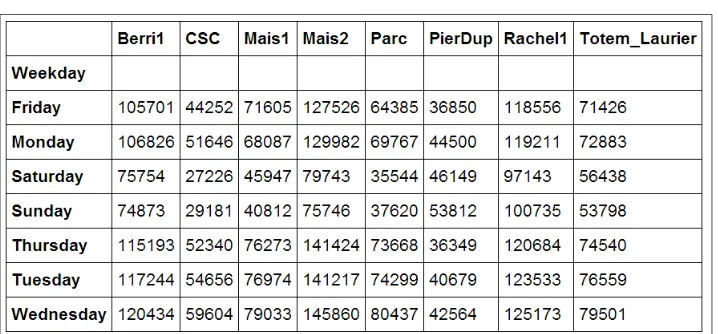
7. Now, we move to a slightly more advanced analysis. We will look at the attendance of all tracks as a function of the weekday. We can get the weekday easily with pandas: the index attribute of the DataFrame object contains the dates of all rows in the table. This index has a few date-related attributes, including weekday:
In [7]: df.index.weekday
Out[7]: array([1, 2, 3, 4, 5, 6, 0, 1, 2, ..., 0, 1, 2])
However, we would like to have names (Monday, Tuesday, and so on) instead of numbers between 0 and 6. This can be done easily. First, we create a days array with all the weekday names. Then, we index it by df.index.weekday. This operation replaces every integer in the index by the corresponding name in days. The first element, Monday, has the index 0, so every 0 in df.index.weekday is replaced by Monday and so on. We assign this new index to a new column, Weekday, in DataFrame:
In [8]: days = np.array(['Monday', 'Tuesday', 'Wednesday', 'Thursday', 'Friday', 'Saturday', 'Sunday'])
df['Weekday'] = days[df.index.weekday]
8. To get the attendance as a function of the weekday, we need to group the table elements by the weekday. The groupby() method lets us do just that. Once grouped, we can sum all the rows in every group:
In [9]: df_week = df.groupby('Weekday').sum() In [10]: df_week
A Tour of Interactive Computing with IPython
9. We can now display this information in a figure. We first need to reorder the table by the weekday using ix (indexing operation). Then, we plot the table, specifying the line width:
In [11]: df_week.ix[days].plot(lw=3)
plt.ylim(0); # Set the bottom axis to 0.
10. Finally, let's illustrate the new interactive capabilities of the notebook in IPython 2.0. We will plot a smoothed version of the track attendance as a function of time (rolling mean). The idea is to compute the mean value in the neighborhood of any day. The larger the neighborhood, the smoother the curve. We will create an interactive slider in the notebook to vary this parameter in real time in the plot. All we have to do is add the @interact decorator above our plotting function:
In [12]: from IPython.html.widgets import interact @interact
def plot(n=(1, 30)):
pd.rolling_mean(df['Berri1'], n).dropna().plot() plt.ylim(0, 8000)
Chapter 1
Interactive widget in the notebook
There's more...
pandas is the right tool to load and manipulate a dataset. Other tools and methods are generally required for more advanced analyses (signal processing, statistics, and mathematical modeling). We will cover these steps in the second part of this book, starting with Chapter 7, Statistical Data Analysis.
Here are some more references about data manipulation with pandas:
f Learning IPython for Interactive Computing and Data Visualization, Packt Publishing, our previous book
f Python for Data Analysis, O'Reilly Media, by Wes McKinney, the creator of pandas f The documentation of pandas available at http://pandas.pydata.org/
pandas-docs/stable/
See also
A Tour of Interactive Computing with IPython
Introducing the multidimensional array in
NumPy for fast array computations
NumPy is the main foundation of the scientific Python ecosystem. This library offers a specific data structure for high-performance numerical computing: the multidimensional array. The rationale behind NumPy is the following: Python being a high-level dynamic language, it is easier to use but slower than a low-level language such as C. NumPy implements the multidimensional array structure in C and provides a convenient Python interface, thus bringing together high performance and ease of use. NumPy is used by many Python libraries. For example, pandas is built on top of NumPy.
In this recipe, we will illustrate the basic concepts of the multidimensional array. A more comprehensive coverage of the topic can be found in the Learning IPython for Interactive Computing and Data Visualization book.
How to do it...
1. Let's import the built-in random Python module and NumPy:
In [1]: import random import numpy as np
We use the %precision magic (defined in IPython) to show only three decimals in the Python output. This is just to reduce the number of digits in the output's text.
In [2]: %precision 3 Out[2]: u'%.3f'
2. We generate two Python lists, x and y, each one containing 1 million random numbers between 0 and 1:
In [3]: n = 1000000
x = [random.random() for _ in range(n)] y = [random.random() for _ in range(n)] In [4]: x[:3], y[:3]
Out[4]: ([0.996, 0.846, 0.202], [0.352, 0.435, 0.531])
3. Let's compute the element-wise sum of all these numbers: the first element of x plus the first element of y, and so on. We use a for loop in a list comprehension:
In [5]: z = [x[i] + y[i] for i in range(n)] z[:3]
Chapter 1
4. How long does this computation take? IPython defines a handy %timeit magic command to quickly evaluate the time taken by a single statement:
In [6]: %timeit [x[i] + y[i] for i in range(n)] 1 loops, best of 3: 273 ms per loop
5. Now, we will perform the same operation with NumPy. NumPy works on
multidimensional arrays, so we need to convert our lists to arrays. The np.array() function does just that:
In [7]: xa = np.array(x) ya = np.array(y) In [8]: xa[:3]
Out[8]: array([ 0.996, 0.846, 0.202])
The xa and ya arrays contain the exact same numbers that our original lists, x and y, contained. Those lists were instances of the list built-in class, while our arrays are instances of the ndarray NumPy class. These types are implemented very differently in Python and NumPy. In this example, we will see that using arrays instead of lists leads to drastic performance improvements.
6. Now, to compute the element-wise sum of these arrays, we don't need to do a for loop anymore. In NumPy, adding two arrays means adding the elements of the arrays component-by-component. This is the standard mathematical notation in linear algebra (operations on vectors and matrices):
In [9]: za = xa + ya za[:3]
Out[9]: array([ 1.349, 1.282, 0.733])
We see that the z list and the za array contain the same elements (the sum of the numbers in x and y).
7. Let's compare the performance of this NumPy operation with the native Python loop:
In [10]: %timeit xa + ya
100 loops, best of 3: 10.7 ms per loop
We observe that this operation is more than one order of magnitude faster in NumPy than in pure Python!
8. Now, we will compute something else: the sum of all elements in x or xa. Although this is not an element-wise operation, NumPy is still highly efficient here. The pure Python version uses the built-in sum() function on an iterable. The NumPy version uses the np.sum() function on a NumPy array:
In [11]: %timeit sum(x) # pure Python %timeit np.sum(xa) # NumPy 100 loops, best of 3: 17.1 ms per loop 1000 loops, best of 3: 2.01 ms per loop
A Tour of Interactive Computing with IPython
9. Finally, let's perform one last operation: computing the arithmetic distance between any pair of numbers in our two lists (we only consider the first 1000 elements to keep computing times reasonable). First, we implement this in pure Python with two nested for loops:
In [12]: d = [abs(x[i] - y[j])
for i in range(1000) for j in range(1000)] In [13]: d[:3]
Out[13]: [0.230, 0.037, 0.549]
10. Now, we use a NumPy implementation, bringing out two slightly more advanced
notions. First, we consider a two-dimensional array (or matrix). This is how we deal with the two indices, i and j. Second, we use broadcasting to perform an operation between a 2D array and 1D array. We will give more details in the How it works... section.
In [14]: da = np.abs(xa[:1000,None] - ya[:1000]) In [15]: da
Out[15]: array([[ 0.23 , 0.037, ..., 0.542, 0.323, 0.473], ...,
[ 0.511, 0.319, ..., 0.261, 0.042, 0.192]]) In [16]: %timeit [abs(x[i] - y[j])
for i in range(1000) for j in range(1000)] %timeit np.abs(xa[:1000,None] - ya[:1000])
1 loops, best of 3: 292 ms per loop 100 loops, best of 3: 18.4 ms per loop Here again, we observe significant speedups.
How it works...
A NumPy array is a homogeneous block of data organized in a multidimensional finite grid. All elements of the array share the same data type, also called dtype (integer, floating-point number, and so on). The shape of the array is an n-tuple that gives the size of each axis.
A 1D array is a vector; its shape is just the number of components.
Chapter 1
The following figure illustrates the structure of a 3D (3, 4, 2) array that contains 24 elements:
A NumPy array
The slicing syntax in Python nicely translates to array indexing in NumPy. Also, we can add an extra dimension to an existing array, using None or np.newaxis in the index. We used this trick in our previous example.
Element-wise arithmetic operations can be performed on NumPy arrays that have the same shape. However, broadcasting relaxes this condition by allowing operations on arrays with different shapes in certain conditions. Notably, when one array has fewer dimensions than the other, it can be virtually stretched to match the other array's dimension. This is how we computed the pairwise distance between any pair of elements in xa and ya.
How can array operations be so much faster than Python loops? There are several reasons, and we will review them in detail in Chapter 4, Profiling and Optimization. We can already say here that:
f In NumPy, array operations are implemented internally with C loops rather than Python loops. Python is typically slower than C because of its interpreted and dynamically-typed nature.
f The data in a NumPy array is stored in a contiguous block of memory in RAM. This property leads to more efficient use of CPU cycles and cache.
There's more...
A Tour of Interactive Computing with IPython
Here are some more references:
f Introduction to the ndarray on NumPy's documentation available at
http://docs.scipy.org/doc/numpy/reference/arrays.ndarray.html
f Tutorial on the NumPy array available at http://wiki.scipy.org/ Tentative_NumPy_Tutorial
f The NumPy array in the SciPy lectures notes present at http://scipy-lectures. github.io/intro/numpy/array_object.html
See also
f The Getting started with exploratory data analysis in IPython recipe
f The Understanding the internals of NumPy to avoid unnecessary array copying recipe in Chapter 4, Profiling and Optimization
Creating an IPython extension with custom
magic commands
Although IPython comes with a wide variety of magic commands, there are cases where we need to implement custom functionality in a new magic command. In this recipe, we will show how to create line and magic cells, and how to integrate them in an IPython extension.
How to do it...
1. Let's import a few functions from the IPython magic system:
In [1]: from IPython.core.magic import (register_line_magic, register_cell_magic)
2. Defining a new line magic is particularly simple. First, we create a function that accepts the contents of the line (except the initial %-prefixed name). The
name of this function is the name of the magic. Then, we decorate this function with @register_line_magic:
In [2]: @register_line_magic def hello(line):
if line == 'french':
print("Salut tout le monde!") else:
Chapter 1
3. Let's create a slightly more useful %%csv cell magic that parses a CSV string and returns a pandas DataFrame object. This time, the arguments of the function are the characters that follow %%csv in the first line and the contents of the cell (from the cell's second line to the last).
In [5]: import pandas as pd
#from StringIO import StringIO # Python 2
We can access the returned object with _.
In [7]: df = _
df.describe() Out[7]:
col1 col2 col3 count 3.000000 3.000000 3.000000 mean 3.333333 4.333333 5.333333 ...
min 0.000000 1.000000 2.000000 max 7.000000 8.000000 9.000000
4. The method we described is useful in an interactive session. If we want to use the same magic in multiple notebooks or if we want to distribute it, then we need to create an IPython extension that implements our custom magic command. The first step is to create a Python script (csvmagic.py here) that implements the magic. We also need to define a special function load_ipython_extension(ipython):
In [8]: %%writefile csvmagic.py import pandas as pd
A Tour of Interactive Computing with IPython
def csv(line, cell): sio = StringIO(cell) return pd.read_csv(sio)
def load_ipython_extension(ipython):
"""This function is called when the extension is loaded. It accepts an
IPython InteractiveShell instance. We can register the magic with the `register_magic_function` method."""
ipython.register_magic_function(csv, 'cell') Overwriting csvmagic.py
5. Once the extension module is created, we need to import it into the IPython session. We can do this with the %load_ext magic command. Here, loading our extension immediately registers our %%csv magic function in the interactive shell:
In [9]: %load_ext csvmagic In [10]: %%csv
col1,col2,col3 0,1,2
3,4,5 7,8,9 Out[10]:
col1 col2 col3 0 0 1 2 1 3 4 5 2 7 8 9
How it works...
An IPython extension is a Python module that implements the top-level load_ipython_ extension(ipython) function. When the %load_ext magic command is called, the module is loaded and the load_ipython_extension(ipython) function is called. This function is passed the current InteractiveShell instance as an argument. This object implements several methods we can use to interact with the current IPython session.
The InteractiveShell class
An interactive IPython session is represented by a (singleton) instance of the
Chapter 1
The list of all methods of InteractiveShell can be found in the reference API (see link at the end of this recipe). The following are the most important attributes and methods:
f user_ns: The user namespace (a dictionary).
f push(): Push (or inject) Python variables in the interactive namespace.
f ev(): Evaluate a Python expression in the user namespace.
f ex(): Execute a Python statement in the user namespace.
f run_cell(): Run a cell (given as a string), possibly containing IPython magic commands.
f safe_execfile(): Safely execute a Python script.
f system(): Execute a system command.
f write(): Write a string to the default output.
f write_err(): Write a string to the default error output.
f register_magic_function(): Register a standalone function as an IPython magic function. We used this method in this recipe.
Loading an extension
The Python extension module needs to be importable when using %load_ext. Here, our module is in the current directory. In other situations, it has to be in the Python path. It can also be stored in ~\.ipython\extensions, which is automatically put in the Python path. To ensure that our magic is automatically defined in our IPython profile, we can instruct IPython to load our extension automatically when a new interactive shell is launched. To do this, we have to open the ~/.ipython/profile_default/ipython_config.py file and put 'csvmagic' in the c.InteractiveShellApp.extensions list. The csvmagic module needs to be importable. It is common to create a Python package that implements an IPython extension, which itself defines custom magic commands.
There's more...
Many third-party extensions and magic commands exist, notably cythonmagic, octavemagic, and rmagic, which all allow us to insert non-Python code in a cell. For example, with cythonmagic, we can create a Cython function in a cell and import it in the rest of the notebook.
Here are a few references:
f Documentation of IPython's extension system available at http://ipython.org/ ipython-doc/dev/config/extensions/
A Tour of Interactive Computing with IPython
f Index of IPython extensions at https://github.com/ipython/ipython/wiki/ Extensions-Index
f API reference of InteractiveShell available at http://ipython.org/
ipython-doc/dev/api/generated/IPython.core.interactiveshell.html
See also
f The Mastering IPython's configuration system recipe
Mastering IPython's configuration system
IPython implements a truly powerful configuration system. This system is used throughout the project, but it can also be used by IPython extensions. It could even be used in entirely new applications.
In this recipe, we show how to use this system to write a configurable IPython extension. We will create a simple magic command that displays random numbers. This magic command comes with configurable parameters that can be set by the user in their IPython configuration file.
How to do it...
1. We create an IPython extension in a random_magics.py file. Let's start by importing a few objects.
Be sure to put the code in steps 1-5 in an external text file named
random_magics.py, rather than in the notebook's input!
from IPython.utils.traitlets import Int, Float, Unicode, Bool from IPython.core.magic import (Magics, magics_class, line_magic) import numpy as np
2. We create a RandomMagics class deriving from Magics. This class contains a few configurable parameters:
@magics_class
class RandomMagics(Magics):
text = Unicode(u'{n}', config=True) max = Int(1000, config=True)
Chapter 1
3. We need to call the parent's constructor. Then, we initialize a random number generator with a seed:
def __init__(self, shell):
super(RandomMagics, self).__init__(shell)
self._rng = np.random.RandomState(self.seed or None)
4. We create a %random line magic that displays a random number:
@line_magic
def random(self, line):
return self.text.format(n=self._rng.randint(self.max))
5. Finally, we register that magic when the extension is loaded:
def load_ipython_extension(ipython): ipython.register_magics(RandomMagics)
6. Let's test our extension in the notebook:
In [1]: %load_ext random_magics In [2]: %random
Out[2]: '635' In [3]: %random Out[3]: '47'
7. Our magic command has a few configurable parameters. These variables are meant to be configured by the user in the IPython configuration file or in the console when starting IPython. To configure these variables in the terminal, we can type the following command in a system shell:
ipython --RandomMagics.text='Your number is {n}.' --RandomMagics. max=10 --RandomMagics.seed=1
In this session, we get the following behavior:
In [1]: %load_ext random_magics In [2]: %random
Out[2]: u'Your number is 5.' In [3]: %random
Out[3]: u'Your number is 8.'
8. To configure the variables in the IPython configuration file, we have to open the ~/.ipython/profile_default/ipython_config.py file and add the following line:
c.RandomMagics.text = 'random {n}'
After launching IPython, we get the following behavior: