Collocated Adaptive Control of Underactuated Mechanical Systems
Daniele Pucci, Francesco Romano, and Francesco Nori
Abstract—Collocated adaptive control of underactuated mechanical sys-tems is still a concern for the control community. The main difficulty comes from the nonlinearity of the collocated inverse dynamics with respect to the base parameters, which forbids the direct application of classical adaptive control schemes. This paper extends and encompasses the Slotine’s adap-tive control, which was developed for fully actuated mechanical systems, to stabilize the collocated state space of an underactuated mechanical system. The key point is to define the sliding variable as the difference between the system’s velocity and an exogenous state whose dynamics is considered as control input. We first revisit the Slotine’s result in view of this definition and then show how to extend it to the underactuated case. Stability and convergence of time-varying reference trajectories for the collocated dy-namics are shown to be in the sense of Lyapunov. Global well-posedness of the control laws is achieved by means of a new algebraic property of the mass matrix. Simulations, comparisons to existing control strategies, and experimental results on a two-link manipulator verify the soundness of the proposed approach.
Index Terms—Adaptive control, collocated control, underactuated me-chanical systems.
I. INTRODUCTION
Feedback control of underactuated mechanical systems is not new to the scientific community (see, e.g., [1]–[3] and the ref-erences therein). Aircraft, underwater vehicles, and humanoid robots are only a few examples where the number of control in-puts is fewer than the system’s degrees of freedom, which char-acterizes the nature of an underactuated system [4]. Clearly, the lack of actuation along with model uncertainties significantly complexify the control problem associated with these systems. Given an open-chain mechanical system, this study proposes control strategies for a subset of the system’s degrees of free-dom by using estimates of its dynamical model. In the language of automatic control, the laws presented in this paper fall into the category ofadaptive control schemes[5].
Underactuated mechanical systems raise specific issues when attempting the control of the entire state space. For instance, assuming that the system’s desired configuration is feasible, the nature of a stabilizing controller for this configuration is intimately related to the nature of the system itself. In particular, mechanical systems without potential terms in general forbid the existence of time-invariant feedback continuous stabilizers [6].
Manuscript received October 17, 2014; revised June 29, 2015; accepted September 18, 2015. Date of publication October 16, 2015; date of current ver-sion December 2, 2015. This work was supported by FP7 EU project CoDyCo under Grant 600716 ICT 2011.2.1 Cognitive Systems and Robotics. This paper was recommended for publication by Associate Editor P.-B. Wieber and Editor T. Murphey upon evaluation of the reviewers’ comments.
The authors are with the Department of Robotics, Brain, and Cogni-tive Sciences, Istituto Italiano di Tecnologia, 16163 Genova, Italy (e-mail: [email protected]; [email protected]; [email protected]).
Color versions of one or more of the figures in this paper are available online at http://ieeexplore.ieee.org.
Digital Object Identifier 10.1109/TRO.2015.2481282
This claim, which follows from an application of Brockett’s Theorem [7], has motivated the development of discontinuous and/or time-varying feedback stabilizers for specific classes of underactuated systems (see, e.g., [8]–[11]).
Complexity of the control problem associated with underac-tuated mechanical systems reduces when attempting to stabilize only a subset of the system’s degrees of freedom. In the special-ized literature, several methods have been proposed to achieve this objective. Inverse dynamics [4], [12], sliding mode [13], and energy-based techniques [14] are among the main tools exploited by these works. The common denominator of these approaches is to partition the set of degrees of freedom into two subsets, usually referred to ascollocatedandnoncollocated. The former, whose cardinality equals the number of control inputs, contains theactuated degrees of freedom. The latter accounts for the remaining nonactuateddegrees; see [4] for additional details. Then, the control objective is usually defined as the asymptotic stabilization of either set to desired values.
To cope with model uncertainties, the adaptive control of generic systems has received much attention from the control community. Most works in the specialized literature make spe-cific assumptions on the relationship between the system’s dy-namics and the set of parameters that characterize it. More pre-cisely, adaptive control of feedback linearizable systems is fea-sible [15]. This work, however, assumes that the dynamics can be expressed linearly with respect to the system’s parameters, and this is not the case for the collocated dynamics of an under-actuated mechanical system. An attempt to the adaptive control of nonlinearly parameterized systems can be found in [16]; but the assumption that there exists a parameter independent input ensuring global stability irrespective of the parameters complex-ifies the application of this theory to our case.
When considering the specific class of mechanical systems, adaptive stabilizations of the collocated and noncollocated dy-namics can be achieved [17]. The main drawback of the ap-proach is that the measurement of the system’s acceleration is required by the feedback action. Leaving aside causality issues, this measurement may not be always available.
In the case of fully actuated mechanical systems, adap-tive stabilization of time-varying reference trajectories can be achieved [18], [19]. The key assumption is that the system’s in-verse dynamics (see [20, p. 54]) can be expressed linearly with respect to a set of constantbase parameters. The extension of these works to the underactuated case is not straightforward. As a matter of fact, the collocated inverse dynamics is no longer linear with respect to the base parameters when expressed inde-pendently from the noncollocated accelerations.
Assuming that the control objective is the asymptotic stabi-lization of the collocated state space, this paper basically extends the Slotine’s adaptive controller [18] to the underactuated case.
Inspired by the back-stepping method, the key point is to view the sliding variable as the difference between the system’s ve-locity and an exogenous state, whose dynamics is considered as control input. We then show that this formulation can en-compass the Slotine’s result [18] for fully actuated mechanical systems. In contrast with [18] and inspired by the work by Spong
et al.[19], we show that stability is in the sense of Lyapunov. The new definition of the sliding variable allows us to extend directly the controller [18] to the underactuated case when the objective is the stabilization of the collocated dynamics. No acceleration measurement is required by the proposed control laws. Simulation results, comparisons to a linear controller and to the approach [17], and experiments carried out on a two-link manipulator verify the soundness of the proposed control laws. The reader must be aware that it is beyond the scope of this work to address the classical, and well-known, drawbacks of adaptive control schemes (see, e.g., [21] and the references therein).
This paper is organized as follows. Section II presents the assumptions and the system’s model for the mechanical system. Section III revisits the Slotine’s adaptive control result [18]. Section IV presents the main theoretical results concerning the extension of [18] to the underactuated case. Validations of the approach are presented in Section V, first through simulations and then through experiments. Remarks and perspectives con-clude the paper.
II. BACKGROUND A. Notation
The following notation is used throughout the paper.
r
The set of real numbers is denoted byR.r
Letuandvbe twon-dimensional column vectors of real numbers, i.e.,u, v∈Rn, their inner product is denoted as x⊤y, with “⊤” the transpose operator.r
Given a time function f(t)∈Rn, its first- and second-order time derivative are denoted by f˙(t) andf¨(t), re-spectively. Given a functionf(·)of several variables, its gradient w.r.t. some of them, sayx, is the row vector de-noted as∂xf.r
The Euclidean norm of either a vector or a matrix of real numbers is denoted by| · |.r
In ∈Rn×n denotes the identity matrix of dimension n; 0n ∈Rn denotes the zero column vector of dimensionn;
0n×m ∈Rn×m is the zero matrix of dimensionn×m.
B. System Modeling and Properties
We assume that the application of Lagrange formulation to the mechanical system yields a model of the following form [20]:
M(q, π)¨q+C(q,q, π˙ ) ˙q+g(q, π)
+Fv(π) ˙q+F(q,q, π˙ ) =τ (1)
where q∈Rn denotes the generalized coordinates of the me-chanical system; M(·)∈Rn×n,C(·)∈Rn×n, and g(·)∈Rn denote the inertia matrix, the Coriolis matrix, and the gravity torques, respectively;π∈Rpis the vector of the (constant) sys-tem’s base parameters [22];Fv ∈Rn×n andF(·)∈Rn model
viscous and nonlinear friction torques (i.e.,Fvis a positive
def-inite matrix); andτ is the vector of control inputs (i.e., desired actuators’ torques) to be designed for achieving specific control objectives.
Hence, we assume that the mechanical system hasnconstant degrees of freedom globally parameterized by the coordinatesq. Consequently, we say that system (1) is “underactuated”1when the number of available torque inputs is smaller thann.
We assume the following properties of the model (1).
Property 1: The inertia matrixMis bounded and symmetric positive definite for anyq, i.e.,
λ1(π)In ≤M(q, π)≤λ2(π)In ∀q
withλ1 andλ2 two strictly positive constants.
Property 2: The matrixM˙ −2Cis skew-symmetric, i.e.,
x⊤( ˙M−2C)x= 0 ∀x∈Rn.
Property 3: The Coriolis matrixC(q,q, π˙ )satisfies
|C(q,q, π˙ )| ≤λ0(π)|q˙| ∀q
for some bounded constantλ0.
Property 4: The gravity vectorg(q, π)satisfies
|g(q, π)| ≤γ0(π) ∀q
for some bounded constantγ0.
Property 5: The model (1) can be expressed linearly with respect to the system’s base parameters π. In addition, there exists aregressor matrixY(·)∈Rn×psuch that
M(q, π)¨q+C(q,q, π˙ )ξ+g(q, π)
+Fv(π)ξ+F(q,q, π˙ ) =Y(q,q, ξ,˙ q¨)π
for any vectorξ∈Rn.
The matrixY(·) is the so-called Slotine–Li regressor. Ob-serve that in view of the algebraic Property 5, dynamics (1) can be compactly written by substituting ξ with q, i.e.,˙
Y(q,q,˙ q,˙ q¨)π=τ. As an example, all above properties hold in the case of rigid robot manipulators [20].
III. REVISITING THESLOTINE’SADAPTIVECONTROL
Letr(t)∈Rn denote a time-varying reference trajectory for the variablesq. Throughout the paper, we assume the following.
Assumption 1: The reference trajectory r(t)is bounded in norm onR+, and its first- and second-order time derivatives are well defined and bounded on this set.
We present below a revisited version of the scheme [18] that ensures the asymptotic stabilization of the tracking error
e:= q−r (2)
to zero without the knowledge of the system’s parameters π. The benefits of the following slightly different formulation will
1For more rigorous definitions of “underactuated mechanical systems,”
be clear in the next section. First, define
where˜πis the base parameters estimation error. By considering
˙ˆ
πandξ˙as auxiliary control inputs, fusing and reformulating the results [18], [19] lead to the following lemma.
Lemma 1: Assume that Properties 1–5 and Assumption 1 hold. Apply the following control laws to system (1)
τ = Y(q,q, ξ,˙ ξ˙)ˆπ−Ks (4a)
˙
ξ= ¨r−Λ1e˙−Λ2e (4b)
˙ˆ
π= −ΓY⊤(q,q, ξ,˙ ξ˙)s (4c)
withK,Λ1,Λ2 ∈Rn×ndiagonal, constant positive-definite ma-trices, andΓ∈Rp×p a constant positive definite matrix. Then, the following results hold.
1) The equilibrium point(e,ξ, s,˜ π˜) = (0n,0n,0n,0p)of the closed-loop dynamics( ˙e,ξ,˙˜s,˙ π˙˜)is stable.
2) For any initial condition(e,ξ, s,˜ π˜)(0), the trajectories of the closed-loop dynamics are bounded, and the tracking error e(t)converges to zero.
The proof is given in Appendix. The main difference between the above formulation and that of [18] resides in the defini-tion (3b), and in the fact thatξ˙is viewed as an auxiliary input. The above lemma shows that this standpoint does not affect sta-bility, in terms of Lyapunov, and convergence. Observe also that boundedness and convergence are independent from the initial conditionξ˜(0)thanks to the additional termΛ2ein (4b). This term plays the role of an integral action in the expression of (3b) and compensates for the initial conditionξ˜(0).
For Lemma 1 to hold, it is assumed that system (1) is fully ac-tuated. The following section proposes an extension of Lemma 1 to the case where system (1) is underactuated.
IV. COLLOCATEDADAPTIVECONTROL
Assume that system (1) possesses onlym < ntorque control inputs so that the firstk:=n−mrows on the right-hand side of (1) are identically equal to zero, i.e.,
Y(q,q,˙ q,˙ q¨)π=
withτ¯∈Rm the control inputs. Now, partition the generalized coordinate vectorqas follows:
q:=
fornoncollocatedandcollocated, respectively. Assume that the control objective is the asymptotic stabilization of the collocated coordinatesqcabout reference trajectoriesr(t)∈Rm, i.e., the
stabilization of the tracking error
e:=qc−r (7)
to zero. As before, we want to design control laws for this control objective without the knowledge of the parametersπ.
To provide the reader with a better comprehension of the genesis of this paper, let us show the difficulties in attempting to apply Lemma 1 for controlling the collocated state spaceqc. This
lemma assumes that Property 5 holds, i.e., the inverse dynamics of the controlled variables is linear with respect to the parameters π. In view of the system dynamics (5), this linearity still holds for the collocated state spaceqc. Then, the stabilization of the
tracking erroreto zero may be achieved by applying the laws (4) as follows:
accelerations of the noncollocated state spaceq¨n. Therefore, if
the measurement of this acceleration were available, one might apply the laws (4) for the adaptive control ofeto zero.
The above approach, which is basically that of [17], does pose causality issues. In fact, the acceleration q¨n in (8a) depends
upon the control input τ¯ via the dynamic equation (1), i.e.,
¨
qn = ¨qn(¯τ). To avoid these causality concerns, one may think
of substituting the acceleration q¨n in (5) with its expression
deduced by the dynamical model (1). However, in this case, it is simple to show that the obtained inverse dynamics
¯
τ= ¯τ(π, q,q,˙ q¨c)
is no longer linear with respect to the base parametersπ, which destroys the stability and convergence arguments of Lemma 1.
The next theorem presents control laws that ensure the adap-tive asymptotic stabilization of the collocated variables without acceleration feedback, thus avoiding causality concerns and cir-cumventing the nonlinearity of the collocated inverse dynamics with respect to the base parameters.
Theorem 1: Assume that Properties 1–5 and Assumption 1 hold. Partition the variablesξas follows:
Apply the following control laws to system (5):
positive-definite matrices, and the matrixMndefined as the
kth-order leading principal minor of the mass matrixM evaluated with estimated base parameters, i.e.,
Mn :=SkM(q,ˆπ)S⊤k (13)
where the selectorSk is given by
Sk := Ik 0k×(n−k). (14)
Then, the following results hold.
1) The equilibrium point(e,ξ˜c, s,π˜) = (0m,0m,0n,0p)of the
closed-loop dynamics( ˙e,ξ˙˜c,s,˙ π˙˜)is stable.
2) Assume that the noncollocated velocities remain bounded, i.e.,∃δ >0such that|q˙n|< δ ∀t. There exists a
neighbor-hoodIof the origin(0m,0m,0n,0p)such that if the initial condition(e,ξ˜c, s,π˜)(0)belongs toI, then the tracking
er-rore(t)converges to zero.
The proof is given in Appendix. The appeal of the invoked reformulation of the Slotine’s adaptive control presented in Lemma 1 lies in the similarity between the control laws (4) and (11) and (12). More precisely, in both cases, the evolution of the variableξcan be obtained by numerical integration of its dynamicsξ. When the system possesses˙ kunactuated degrees of freedom, it suffices to modify the firstkelements of this dy-namics —see (11b)—to still ensure stability and convergence of the collocated coordinates. Note that the dynamicsξ˙n in (11b)
plays the role of an estimator for the noncollocated acceleration
¨
qn when the system’s trajectories belong to a neighborhood of
the equilibrium point.
Convergence of the tracking error e to zero is guaran-teed, however, when the noncollocated velocities |q˙n|remain
bounded. This requirement, which follows from the application of Barbalat’s lemma, is reminiscent of the condition on the sta-bility of the zero dynamics in [15]. Let us remark that stasta-bility is here guaranteed independently from the boundedness ofq˙n,
which cannot be in general satisfied by an appropriate choice of the control inputτ. In fact, the influence of this input on the¯
noncollocated dynamics cannot be guaranteed to have general properties. Clearly, friction effects may play a role in guarantee-ing the boundedness of|q˙n|and, consequently, the convergence
of the tracking errore(t)to zero.
A. Desingularization for a Globally Defined Controller
The local nature of the controls (11) is due to the fact that ma-trix (13) may not be invertible far from the pointπ˜=0p. Observe that the invertibility of (13) in a neighborhood of this point is
guaranteed by Property 1, which implies that each leading prin-cipal minor of the mass matrixM(q, π)is positive definite and, therefore, invertible.
The noninvertibility of the matrix (13) is related to the stan-dard inertial parameters2associated with the estimated base pa-rametersπ. For instance, when an estimateˆ ˆπinduces a negative mass of a rigid body composing the underlying mechanical sys-tem, the inertia matrixM(q,πˆ)may not be positive definite [24], thus eventually resulting in an ill-conditioned controller. Now, let us remark that if
det (Mn(q(t),πˆ(t)))>0 ∀t (15)
independently of the initial conditions, laws (11) ensure global convergence of the tracking error and global boundedness. This may not be always the case, however. To avoid a possible ill-conditioning of the laws (11), a desingularization policy must be defined when the above determinant gets close to zero. The desingularization policy used in this paper exploits the following result on the inertia matrixM(q, π).
Lemma 2: Properties 1 and 5 imply that
[∂πdet (SiM(q, π)Si⊤)]π=idet(SiM(q, π)Si⊤) (16)
∀i∈ {1, . . . , n}and withSigiven by (14). Then, the gradient
with respect toπof the determinant of each leading principal minor of the mass matrixM(q, π)has a norm different from zero, i.e., there existsγ >0such that
|∂πdet (SiM(q, π)Si⊤)|> γ. (17)
The proof is in Appendix. The above lemma in turn implies that there exists a choice forπ˙ˆsuch that the time derivative of (15) can be imposed at will. Then it is theoretically possible to modify the law (12) to ensure that the determinant ofMn
never decreases below a certain threshold. The next proposition presents such a modification of the adaptation lawπ.˙ˆ
Proposition 1. Consider the laws (11) with the adaptation law redefined as follows:
2The standard inertial parameters of a rigid body consist in a 10-D vector
whereε∈R+,
YMn := Sk
Y
q,0n,0n, ei
0m
−Y(q,0n,0n,0n)
(20a)
Υ := (υ1, . . . , υi, . . . , υk) (20b)
υi :=
∂
∂q(YMnπˆ)
˙
q−YMnΓY
⊤(q,q, ξ,˙ ξ˙)s
(20c)
and ei∈Rk denotes a vector of k zeros except for the ith
coordinate, which is equal to 1. Then, the following results hold. 1) IfdetMn
>0, then
|δ|>0 and |ˆπ|>0.
2) Assume thatdetMn
(0)> ε. Then
detMn
(t)≥ε ∀t.
The proof is in Appendix. This proposition states that it is always possible to maintain the determinant of Mn above a
certain thresholdε. In fact, the desingularizing termη in (19) would be ill-conditioned only at|δ|= 0, but this never occurs provided that det (Mn)>0 —see result 1. When compared
with existing desingularization procedures, the main advantage of the above policy is that it does not affect the instantaneous value of the control torqueτ, but only its derivative with respect¯
to time. This characteristic is of a pivotal role in practice since it helps minimize the additional effort that the actuators must withstand close to the ill-conditioning point of the control laws. In light of the above, the always-defined control laws are given by (11)–(18). Clearly, the larger the thresholdε, the larger the influence of the desingularizing termηδ on the results of Theorem 1. Consequently, this threshold must be tuned depend-ing on the specific system. Assumdepend-ing that one is given with best guessesπ¯ of the system’s base parametersπ, we suggest to setε= det(M(¯q,¯π)), with q¯a tunable parameter. For in-stance, ifr(t)converges to some desired valuesrd, one may set ¯
q= (q⊤
n(0), rd⊤)⊤. Simulations and experimental results
pre-sented next show that the influence of this desingularizing term ηδdoes not significantly affect the practical stability and bound-edness of the tracking errore.
Remark 1: Dynamics (1) assumes that no external wrench acts on the system. The effects of an external measurable wrench wecan be modeled as a disturbanced:=J⊤(q)we ∈Rn, with
J(q)the Jacobian of the frame associated with the application point of the wrenchwe. The termdmust be then added on the
right-hand side of (1). Now, partitiond=d⊤
n d⊤c
⊤ , where dn ∈Rk anddc∈Rm. To retain stability and convergence of
the collocated variables, it suffices to apply (11) and (18) with
¯
τ=Yc(q,q, ξ,˙ ξ˙)ˆπ−Ksc−dc
˙
ξn =Mn−1
Knsn+dn−Yn
q,q, ξ,˙
0k ˙
ξc
ˆ
π
.
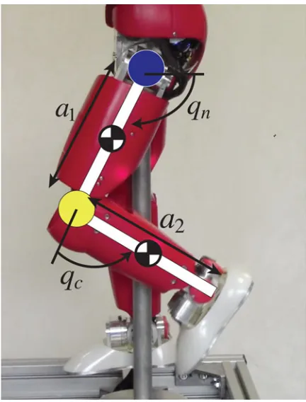
Fig. 1. Two-link manipulator obtained from the iCub’s leg.
V. SIMULATIONS ANDEXPERIMENTALRESULTS
In this section, we test the control laws (11)–(18) first through simulations and then through experiments carried out on a two-link manipulator with rotational joints.
The 2R manipulator is obtained from thehip—nonactuated joint—and the knee—actuated joint—of the iCub humanoid robot (see Fig. 1). The robot’s ankle is kept fixed with a position controller. When applied to this case study, the laws (11)–(18) require the regressor Y(·) of a two-link manipulator [25, p. 268]. This regressor is computed with only viscous friction terms, which play a role when the controller is launched on the real robot. More precisely, the iCub platform is equipped with a low-level torque control loop that is in charge of stabilizing
any desired joint torque [26], [27]. This loop is supposed to compensate for friction effects, but this compensation is never perfect. Therefore, the friction terms Fvq˙ left in the regressor
can account for imperfect viscous friction compensations by the low-level torque control.
Simulations are performed with the following parameters: ml1 =ml2 = 2 [kg], Il1 =Il2 = 0.2528 [kg m
2], l
1 =l2 = 0.75 [m], a1=a2 = 1.5 [m], Fv =I2 [N m s/rad], where (ml1, ml2), (Il1, Il2), (l1, l2), (a1, a2) stand for the masses,
inertias, center-of-mass positions, and lengths of the two links, respectively (see Fig. 1). The associated base parameters are π= [2,−1.5,1.3778,2,−1.5,1.3778,1,1] (see [25, p. 268] with zero motor masses), where the last two elements ofπare the diagonal of the matrixFv. The control inputτ¯is saturated
Fig. 2. Performances of the control laws (11)–(18).
Fig. 2 depicts the simulation result for the reference trajectory
r(t) =π 2
1 + sin(πt)
when the laws (11)–(18) are evaluated with Λ1=Λ2=K=I2, Γ=I8, ε=1.5, and πˆ(0)= (1.8,−1,0.8,2.6,−2,1.7,0.9,1.1).
Convergence of the tracking error is achieved with an overshoot of25◦.
As for elements of comparison with existing control tech-niques, Fig. 4 shows simulation results when applying the law (8) and the laws (11)–(18) with no feedforward term (i.e., Yc(q,q, ξ,˙ ξ˙)ˆπ≡0), which result in a PID controller for all in-tents and purposes. The accelerationq¨nin (8) was estimated by
using a filter of the form s′
(2πf s′+ 1)
wheres′is the Laplace variable, andfis the cutoff frequency of the filter set at10 [Hz]. By doing so, we basically compare our control strategy with that of [17]. Initial conditions, gains, and reference trajectory were kept equal to those associated with the simulation of Fig. 2.
Interestingly, Fig. 4 shows that the lack of the feedforward term Yc(q,q, ξ,˙ ξ˙)ˆπ significantly worsens not only the steady state, but also the transient response. Increasing the PID’s gains would reduce the error in this case, but would result in amplify-ing eventual measurement errors and noises.
Fig. 4 also shows that the law (8) evaluated with an estimated accelerationq¨n renders the variableqcunstable. This instability
is the combined effect of the torque saturation and the cutoff frequency of the filter used to estimate the accelerationq¨n.
Sim-ulations we have performed tend to show that increasing the cutoff frequency reduce the likelihood of rendering the actu-ated variable unstable, but this may be problematic in practice because of well-known issues such as high-frequency noise. Analogously, we verified that increasing the torque saturation would solve the instability problem, but this threshold may not be exceeded in practice.
We then went one step further and applied the laws (11)–(18) to the aforementioned robot obtained from the iCub’s leg. The
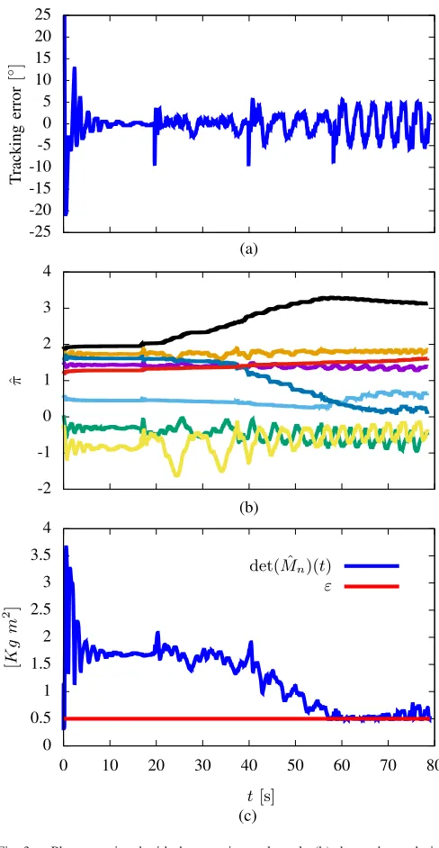
Fig. 3. Plots associated with the experimental result. (b) shows the evolution ofπˆ. Parameters are given with the following color order: purple, green, light blue, orange, yellow, dark blue, red, black, which correspond toˆπ1, . . . ,πˆp.
reference trajectory was chosen as
r(t) =π
4 sin(2πfr(t)t)−
π
3
with a piecewise constant frequencyfr(t)given by
fr(t) =
⎧ ⎪ ⎪ ⎪ ⎪ ⎨ ⎪ ⎪ ⎪ ⎪ ⎩
0Hz, 0 s≤t <20 s 0.1Hz, 20 s≤t <40 s 0.2Hz, 40 s≤t <58 s 0.3Hz, 58 s≤t <80 s.
(4)
Fig. 4. Performances of a PID and the control law (8).
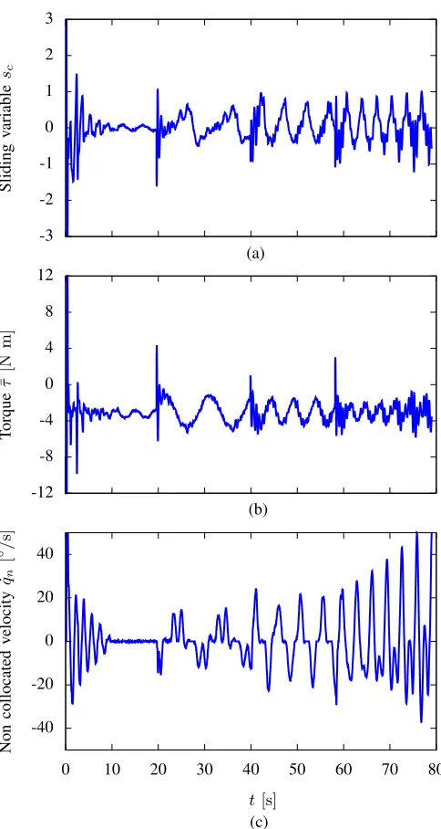
From top to bottom, Figs. 3 and 5 depict the tracking errore, the estimated base parametersπ, the determinant of the matrixˆ
Mn(q,πˆ), the sliding variable sc, the torque control inputτ¯,
and the velocityq˙n of the noncollocated variable. Observe that
the tracking error converges to zero for a constant referencer. Sharp variations of the tracking error and of the torque at the time instantst= 20 [s],t= 40 [s], andt= 58 [s]are due to the discontinuities of the reference trajectoryr(t). Note also that unmodeled friction effects and imperfect tracking of the low-level torque control loop reflect inq˙n = 0 close tot= 20 [s]
[see Fig. 5(c)]. As the frequencyfrincreases, the tracking error
is kept relatively small despite a significant increase of the hip velocity (peak hip velocity at40 [◦/s]). The fact that the tracking error does not converge to zero is mainly due to the imperfect tracking of the low-level torque control loop implemented on the iCub platform.
Fig. 3(c) shows the effects of the desingularization policy defined in Proposition 1. Once above the thresholdε, the de-terminant of Mn(q(t),πˆ(t))never goes below this threshold.
Observe that this desingularization action is of particular im-portance for high-frequency reference trajectories, where the coupling effects between the collocated and noncollocated joints are no longer negligible. Although stability and convergence are not guaranteed when the desingularization action is active, the estimated parameters remain bounded ont∈(60,80) [s][see Fig. 3(b)].
VI. CONCLUSION ANDPERSPECTIVES
We have presented an extension of the Slotine’s adaptive control [18], which was developed for fully actuated manip-ulators, to stabilize the collocated space of an underactuated mechanical system. Stability and convergence of the collocated variables were shown by using Lyapunov and Barbalat argu-ments. Compared with existing results, our approach does not make use of any acceleration measurement, thus avoiding al-together causality concerns. The control results were validated with simulations, comparisons, and with an implementation on a two-link manipulator obtained from the iCub humanoid robot. It was beyond the scope of this study to address the classical, and well-known, drawbacks of adaptive control schemes [21].
Fig. 5. Plots associated with the experimental result.
presented approach to make iCub walk, where joint trajectories are provided by independent planning algorithms.
The laws presented in this paper render the associated equi-librium point stable, but convergence of the tracking errors is shown when the initial conditions belong to a neighborhood of the equilibrium point. This local nature is due to the fact that the control laws make use of the invertibility of the system’s inertia matrix along the estimated system’s model. This matrix may not be invertible for physical inconsistentbase parame-ters [24]. Then, our goal is to design an estimation dynamics such that the associated base parameters are always physical consistent. In this case, the control laws presented in this paper would guarantee global boundedness and convergence.
APPENDIX
PROOF OFLEMMA1
Consider the following candidate Lyapunov function:
V := 1 andΛ1KΛ−12 are diagonal and positive-definite matrices. In view of Properties 2 and 5, the controls (4a)–(4c), andξ˜=ξ−r˙, one verifies that the time derivative of (22) yields
˙
V = −s⊤Ks−s⊤F
vs+ 2e⊤KΛ1e˙ (23) + 2( ˙r−Λ1e−ξ)⊤Λ1Ke.
Recall thatFvis a positive-definite matrix. From (4b), observe that the variableξcan be obtained by integration, i.e.,
ξ(t) = ˙r−Λ1e−Λ2ζ in the first term on the right-hand side of (23), one has
˙
V = −( ˙e+ Λ2ζ)⊤K( ˙e+ Λ2ζ)−s⊤Fvs−e⊤Λ1KΛ1e. (24) As a consequence,V˙ ≤0. Then, the stability of
(e,ξ, s,˜ π) = (0˜ n,0n,0n,0p)
and the boundedness of the closed-loop trajectories for any initial con-dition follow [30, Th. 4.8, p. 151].
To show that the tracking erroreconverges to zero, let us first prove thatV˙ converges to zero. By direct calculations, one verifies that
¨
V = −2( ˙e+ Λ2ζ)⊤K(¨e+ Λ2e)−2s⊤Fvs˙−2e⊤Λ1KΛ1e.˙ By using Assumption 1, Properties 1, 3, 4, and the fact that the variables
e, ξ, s,π˜are bounded, one deduces thatV¨is bounded. This implies that
˙
V is uniformly continuous, and the application of Barbalat’s Lemma ensures thatV˙ tends to zero. In view of (24), this implies that the error
e(t)converges to zero.
PROOF OFTHEOREM1
Thanks to the formulation of the control result of Lemma 1, this proof is similar to that above. In particular, reconsider the candidate Lyapunov function (22) with ξ˜c:=ξc−r˙ instead ofξ˜. In view of Properties 2 and 5 and the partitioning (10), the application of the controls (11), (12) renders the time derivative ofV as follows:
˙ Given Property 1, note that the auxiliary control inputξ˙nis well defined in a neighborhood of˜π= 0psince each leading principal minor of the mass matrixM(q, π)is invertible whenπˆbelongs to a neighborhood ofπ. As a consequence, the choice of the auxiliary control inputξ˙n in (11b) implies that
In view of (10) and of the above equation, the expression ofV˙ in (25) becomes
Analogously to the proof of Lemma 1, the variableξc(t)can be obtained by integration, i.e.,
ξc(t) = ˙r−Λ1e−Λ2 t
0
e(z)dz−α= ˙r−Λ1e−Λ2ζ
with the collocated erroregiven by (7). Now, by substituting
sc = ˙qc−ξc = ˙e+ Λ1e+ Λ2ζ in the second term on the right-hand side ofV˙, one obtains
˙ V = −sT
nKnsn −( ˙e+ Λ2ζ)⊤K( ˙e+ Λ2ζ) (26)
−s⊤F
vs−e⊤Λ1KΛ1e≤0. Then, the stability of the equilibrium point
(e,ξ˜c, s,π) = (0˜ m,0m,0n,0p)
follows, which clearly implies the boundedness of the system’s tra-jectories when the initial conditions belong to a neighborhood of the equilibrium point.
Given Assumption 1, Properties 1, 3, 4, and the assumption that the noncollocated velocityq˙n remains bounded, it is possible to verify that
¨
V is bounded when the initial conditions belong to a neighborhood of the equilibrium point. Then,V˙ is uniformly continuous, and anal-ogously to the proof of Lemma 1, one shows thate(t) converges to zero.
PROOF OFLEMMA2 First, define
Mi(q, π) :=SiM(q, π)S⊤i ∈Ri×i
withSigiven by (14), as the symmetric positive-definite leading minor of orderiof the mass matrixM(q, π). Then, observe that
M(q, π)¨q:= YM(q,q)π¨
Letej∈Ridenote the vector ofizeros except for thejth coordinate, which is equal to 1. By using Jacobi’s formula,3one has
∂πdet(Mi) = det(Mi)tr(Mi−1∂πMi)
Then, in view of (27), one obtains
∂πdet(Mi) = det(Mi)
Since the inertia matrixMis positive definite, then
det(Mi)>0 ∀i={1, . . . , n}.
This, in turn, implies that
∃γ >0such that|∂πdet (SiM(q, π)S⊤i)|> γ.
PROOF OFPROPOSITION1 Proof of 1): If
det (Mn)>0
then the matrixM−1
n exists. Note thatMnis symmetric by construction. Then, analogously to the proof of the Lemma 2, multiplying (19b) times
ˆ
Since the system is underactuated, thenk≥1. Consequently,|δ|>0
and|πˆ|>0.
Proof of 2):Consider the following storage function:
Vd:=
1 2det
2(M
n).
3Although the Jacobi’s formula is usually applied to a single-parameter
depen-dent matrix, it is possible to verify that the above application to a multi-variable dependent matrix is correct.
It is possible to verify that the time derivative ofVdis
˙
[1] P. X. M. La Hera, “Underactuated mechanical Systems: Contributions to trajectory planning, analysis, and control,” Ph.D. dissertation, Dept. Appl. Phys. Electron., Ume˚aUniv., Ume˚a, Sweden, 2011.
[2] Y. Liu and H. Yu, “A survey of underactuated mechanical systems,” Con-trol Theory Appl., IET, vol. 7, pp. 921–935, Feb. 2013.
[3] R. Olfati-Saber, “Nonlinear control of underactuated mechanical systems with application to robotics and aerospace vehicles,” Ph.D. dissertation, Dept. Elect. Eng. Comput. Sci., Massachusetts Inst. Technol., Cambridge, MA, USA, 2000.
[4] M. W. Spong, “Underactuated mechanical systems,” inControl Problems in Robotics and Automation(Lecture Notes in Control and Information Sciences). New York, NY, USA: Springer, 1998, pp. 135–150.
[5] K. J. Astrom and B. Wittenmark,Adaptive Control, Boston, MA, USA: Addison-Wesley, 1994.
[6] M. Reyhanoglu, A. van der Schaft, N. H. McClamroch, and I. Kol-manovsky, “Dynamics and control of a class of underactuated mechanical systems,”IEEE Trans. Autom. Control, vol. 44, no. 9, pp. 1663–1671, Sep. 1999.
[7] R. Brockett, “Asymptotic stability and feedback stabilization,” Differen-tial Geometric Control Theory, vol. 27, pp. 181–191, 1983.
[8] A. De Luca, R. Mattone, and G. Oriolo, “Dynamic mobility of redundant robots using end-effector commands,” inProc. IEEE Int. Conf. Robot. Autom., pp. 1760–1767, Apr. 1996.
[9] J. Ghommam, F. Mnif, and N. Derbel, “Global stabilisation and track-ing control of underactuated surface vessels,”IET Control Theory Appl., vol. 4, no. 1, pp. 71–88, Jan. 2010.
[10] J. Grizzle, C. Moog, and C. Chevallereau, “Nonlinear control of mechan-ical systems with an unactuated cyclic variable,”IEEE Trans. Autom. Control, vol. 50, no. 5, pp. 559–576, May 2005.
[11] M.-S. Park and D. Chwa, “Swing-up and stabilization control of inverted-pendulum systems via coupled sliding-mode control method,”IEEE Trans. Ind. Electron., vol. 56, no. 9, pp. 3541–3555, Sep. 2009.
[12] A. De Luca and G. Oriolo, “Motion planning and trajectory control of an underactuated Three-Link robot via feedback linearization,” inProc. IEEE Int. Conf. Robot. Autom., 2000, pp. 2789–2795.
[13] R. Santiesteban and T. Floquet, “Second-order sliding mode control of underactuated mechanical systems II: Orbital stabilization of an inverted pendulum with application to swing up/balancing,”Int. J. Robust Nonlin-ear Control, vol. 18, pp. 544–556, 2008.
[14] M. W. Spong, “Energy based control of a class of underactuated mechan-ical systems,” inProc. IFAC World Cong., 1996, pp. 431–435.
[15] S. S. Sastry and A. Isidori, “Adaptive control of linearizable systems,” IEEE Trans. Autom. Control, vol. 34, no. 11, pp. 1123–1131, Nov. 1989. [16] Z. Qu, R. A. Hull, and J. Wang, “Globally stabilizing adaptive control de-sign for nonlinearly-parameterized systems,”IEEE Trans. Autom. Control, vol. 51, no. 6, pp. 1073–1079, Jun. 2006.
[17] Y.-l. Gu and Y. Xu, “Under-actuated robot systems: Dynamic interaction and adaptive control,” inProc. IEEE Int. Conf. Syst. Man Cybern., 1994, vol. 1, pp. 958–963.
[18] J.-J. E. Slotine and W. Li, “Adaptive manipulator control: A case study,” IEEE Trans. Autom. Control, vol. 33, no. 11, pp. 995–1003, Nov. 1988. [19] M. W. Spong, R. Ortega, and R. Kelly, “Comments on, “Adaptive
[20] B. Siciliano and O. Khatib,Handbook of Robotics, vol. 6. New York, NY, USA: Springer, 2008.
[21] B. D. O. Anderson, “Failures of adaptive control theory and their resolu-tion,”Commun. Inf. Syst., vol. 5, pp. 1–20, 2005.
[22] W. Khalil and E. Dombre,Modeling, Identification and Control of Robots. London, U.K.: Butterworth-Heinemann, 2004.
[23] R. Tedrake,Underactuated Robotics: Learning, Planning, and Control for Efficient and Agile Machines: Course Notes for MIT 6.832.Working draft edition, 2009.
[24] K. Yoshida and W. Khalil, “Verification of the positive definiteness of the inertial matrix of manipulators using base inertial parameters,”Int. J. Robot. Res., vol. 19, no. 5, pp. 498–510, May 2000.
[25] B. Siciliano, L. Sciavicco, L. Villani, and G. Oriolo,Robotics: Modelling, Planning and Control. New York, NY, USA: Springer, 2009.
[26] M. Fumagalli, M. Randazzo, F. Nori, L. Natale, G. Metta, and G. Sandini, “Exploiting proximal F/T measurements for the iCub active compliance,” inProc. IEEE/RSJ Int. Conf. Intell. Robots Syst., Oct. 2010, pp. 1870– 1876.
[27] M. Fumagalli, S. Ivaldi, M. Randazzo, L. Natale, G. Metta, G. San-dini, and F. Nori, “Force feedback exploiting tactile and proximal force/torque sensing,” Auton. Robots, vol. 33, no. 4, pp. 381–398, Apr. 2012.
[28] H. Wang, “On adaptive inverse dynamics for free-floating space manipu-lators,”Robot. Auton. Syst., vol. 59, no. 10, pp. 782–788, 2011. [29] R. Featherstone,Rigid Body Dynamics Algorithms. Secaucus, NJ, USA:
Springer-Verlag, 2007.