Improving Cluster Analysis by Co-initializations
He Zhang∗, Zhirong Yang, Erkki Oja
Department of Information and Computer Science, Aalto University, Espoo, Finland
Abstract
Many modern clustering methods employ a non-convex objective function and use iterative optimization algorithms to find local minima. Thus initialization of the algorithms is very important. Conventionally the starting guess of the iterations is randomly chosen; however, such a simple initialization often leads to poor clusterings. Here we propose a new method to improve cluster analy-sis by combining a set of clustering methods. Different from other aggregation approaches, which seek for consensus partitions, the participating methods in our method are used consequently, providing initializations for each other. We present a hierarchy, from simple to comprehensive, for different levels of such co-initializations. Extensive experimental results on real-world datasets show that a higher level of initialization often leads to better clusterings. Especially, the proposed strategy is more effective for complex clustering objectives such as our recent cluster analysis method by low-rank doubly stochastic matrix de-composition (called DCD). Empirical comparison with three ensemble clustering methods that seek consensus clusters confirms the superiority of improved DCD using co-initialization.
Keywords: Clustering, Initializations, Cluster ensembles
∗Corresponding author.
1. Introduction
1
Cluster analysis plays an essential role in machine learning and data min-2
ing. The aim of clustering is to group a set of objects in such a way that the 3
objects in the same cluster are more similar to each other than to the objects 4
in other clusters, according to a particular objective. Many clustering meth-5
ods are based on objective functions which are non-convex. Their optimization 6
generally involves iterative algorithms which start from an initial guess. Proper 7
initialization is critical for getting good clusterings. 8
For simplicity, random initialization has been widely used, where a start-9
ing point is randomly drawn from a uniform or other distribution. However, 10
such a simple initialization often yields poor results and the iterative clustering 11
algorithm has to be run many times with different starting points in order to 12
get better solutions. More clever initialization strategies are thus required to 13
improve efficiency. 14
Many ad hoc initialization techniques have been proposed for specific clus-15
tering methods, for example, specific choices of the initial cluster centers of the 16
classicalk-means method (see e.g. [1, 2, 3, 4]), or singular value decomposition 17
for clustering based on nonnegative matrix factorization [5, 6]. However, there 18
seems to be no initialization principle that would be commonly applicable for a 19
wide range of iterative clustering methods. Especially, there is little research on 20
whether one clustering method can benefit from initializations by the results of 21
another clustering method. 22
In this paper, we show experimentally that the clusterings can usually be 23
improved if a set of diverse clustering methods provide initializations for each 24
other. We name this approachco-initialization. We present a hierarchy of ini-25
tializations towards this direction, where a higher level represents a more exten-26
sive strategy. At the top are two levels of co-initialization strategies. We point 27
out that despite their extra computational cost, these strategies can often bring 28
significantly enhanced clustering performance. The enhancement is especially 29
Latent Semantic Indexing [7], and our recent clustering method by low-rank 31
doubly stochastic matrix decomposition (called DCD) [8]. 32
Our claims are supported by extensive experiments on nineteen real-world 33
clustering tasks. We have used a variety of datasets from different domains 34
such as text, vision, and biology. The proposed initialization hierarchy has been 35
tested using eight state-of-the-art clustering methods. Two widely used crite-36
ria, cluster purity and Normalized Mutual Information, are used to measure 37
the clustering performance. The experimental results verify that a higher level 38
initialization in the proposed hierarchy often achieve better clustering perfor-39
mance. 40
Ensemble clustering is another way to combine a set of clustering methods. 41
It aggregates the different clusterings into a single one. We also compared co-42
initialization with three prominent ensemble clustering methods. The compar-43
ison results show that the improved DCD using co-initializations outperforms 44
these ensemble approaches that seek a consensus clustering. 45
In the following, Section 2 reviews briefly the recently introduced Data-46
Cluster-Data (DCD) method. It is a representative clustering method among 47
those that strongly benefit from co-initializations, and will be shown to be over-48
all the best method in the experiments. Then Section 3 reviews related work 49
on ensemble clustering, which is another way of combining a set of base clus-50
tering methods. In Section 4, we present our novel co-initialization method 51
and describe the initialization hierarchy. Experimental settings and results are 52
reported in Section 5. Section 6 concludes the paper and discusses potential 53
future work. 54
2. Clustering by DCD
55
Some clustering methods such as Normalized Cut [9] are not sensitive to 56
initializations but tend to return less accurate clustering (see e.g. [10], page 8, [8, 57
11], and Section 5.3). On the other hand, some methods can find more accurate 58
more from our co-initialization strategy, to be introduced in Section 4. Recently 60
we proposed a typical clustering method of the latter kind, which is based 61
on Data-Cluster-Data random walk and thus called DCD [8]. In this section 62
we recapitulate the essence of DCD. It belongs to the class of probabilistic 63
clustering methods. Givenndata samples andrclusters, denote byP(k|i) the 64
probability of assigning theith sample to the kth cluster, where i = 1, . . . , n
65
andk= 1, . . . , r. 66
Suppose the similarities between data items are precomputed and given in 67
ann×nnonnegative symmetric sparse matrixA. DCD seeks an approximation 68
to A by another matrix Ab whose elements correspond to the probabilities of 69
two-step random walks between data points through clusters. Let i, j, and v
70
be indices for data points, and k and l for clusters. Then the random walk 71
probabilities are given as 72
The approximation is given by the Kullback-Leibler (KL-) divergence. This 74
is formulated as the following optimization problem [8]: 75
∇+ and∇− are the positive and (unsigned) negative parts of ∇, respectively.
78
The optimization is solved by a Majorization-Minimization algorithm [12, 13, 79
whereai=X
The preprocessing of DCD employs the common approximation of making 82
A sparse by zeroing the non-local similarities. This makes sense for two rea-83
sons: first, geodesics of curved manifolds in high-dimensional spaces can only be 84
approximated by Euclidean distances in small neighborhoods; second, most pop-85
ular distances computed of weak or noisy indicators are not reliable over long 86
distances, and the similarity matrix is often approximated by the K-nearest 87
neighbor graph with good results, especially whennis large. With a sparseA, 88
the computational cost of DCD isO(|E| ×r) for |E|nonzero entries in Aand 89
rclusters. In the experiments we used symmetrized and binarized K-Nearest-90
Neighbor graph asA(K≪n). Thus the computational cost isO(nKr). 91
Given a good initial decomposing matrix P, DCD can achieve better clus-92
ter purity compared with several other state-of-the-art clustering approaches, 93
especially for large-scale datasets where the data points situate in a curved 94
manifold. Its success comes from three elements in its objective: 1) the approx-95
imation error measure by Kullback-Leibler divergence takes into account sparse 96
similarities; 2) the decomposing matrix P as the only variable to be learned 97
contains just enough parameters for clustering; and 3) the decomposition form 98
ensures relatively balanced clusters and equal contribution of each data sample. 99
What remains is how to get a good starting point. The DCD optimization 100
problem is harder to solve than conventional NMF-type methods based on Eu-101
clidean distance in three aspects: 1) the geometry of the KL-divergence cost 102
function is more complex; 2) DCD employs a structural decomposition whereP
103
appears more than once in the approximation, and appears in both numerator 104
and denominator; 3) each row ofP is constrained to be in the (r−1)-simplex. 105
Therefore, finding a satisfactory DCD solution requires more careful initializa-106
tion. Otherwise the optimization algorithm can easily fall into a poor local 107
minimum. 108
Yang and Oja [8] proposed to obtain the starting points by pre-training 109
DCD with regularization term (1−α)PiklogPik. This corresponds to imposing
Dirichlet priors over the rows ofP. By varyingα, the pre-training can provide 111
different starting points for multiple runs of DCD. The final result is given by 112
the one with the smallest DCD objective of Eq. 2. This initialization strategy 113
can bring improvement for certain datasets, whereas the enhancement remains 114
mediocre as it is restricted to the same family of clustering methods. In the 115
remaining, we investigate the possibility to obtain good starting points with the 116
aid of other clustering methods. 117
3. Ensemble clustering
118
In supervised machine learning, it is known that combining a set of classifiers 119
can produce better classification results (see e.g. [16]). There have been also 120
research efforts with the same spirit in unsupervised learning, where several 121
basic clusterings are combined into a single categorical output. The base results 122
can come from results of several clustering methods, or the repeated runs of a 123
single method with different initializations. In general, after obtaining the bases, 124
a combining function, calledconsensus function, is needed for aggregating the 125
clusterings into a single one. We call such aggregating methodsensemble cluster
126
analysis. 127
Several ensemble clustering methods have been proposed. An early method 128
[17] first transforms the base clusterings into a hypergraph and then uses a 129
graph-partitioning algorithm to obtain the final clusters. Gionis and Mannila 130
[18] defined the distance between two clusterings as the number of pairs of ob-131
jects on which the two clusterings disagree, based on which they formulated 132
the ensemble problem as the minimization of the total number of disagreements 133
with all the given clusterings. Fred and Jain [19] explored the idea of evidence 134
accumulation and proposed to summarize various clusterings in a co-association 135
matrix. The incentive of their approach is to weight associations between sam-136
ple pairs by the number of times they co-occur in a cluster from the set of 137
given clusterings. After obtaining the co-association matrix, they applied the 138
[20] introduced new methods for generating two link-based pairwise similarity 140
matrices called connected-triple-based similarity and SimRank-based similarity. 141
They refined similarity matrices by considering both the associations among 142
data points and those among clusters in the ensemble using link-based similar-143
ity measures. In their subsequent work [21], Iam-On et al. released a software 144
package called LinkCluE for their link-based cluster ensemble framework. New 145
approaches that better exploit the nature of the co-association matrix have re-146
cently appeared (see e.g. [22, 23]). 147
Despite the rationales for aggregation, the above methods can produce mediocre 148
results if many base clustering methods fall into their poor local optima during 149
their optimization. Seeking a consensus partition of such bases will not bring 150
extraordinary improvement. To overcome this, in the following we present a 151
new technique that enhances the participating clustering methods themselves. 152
In the experimental part we show that our approach outperforms three well-153
known ensemble clustering methods. 154
4. Improving clustering by co-initializations
155
We consider a novel approach that makes use of a set of existing clustering 156
methods. Instead of combining for consensus partitions, the proposed approach 157
is based on two observations: 1) many clustering methods that use iterative 158
optimization algorithms are sensitive to initializations; random starting guesses 159
often lead to poor local optima; 2) on the other hand, the iterative algorithms 160
often converge to a much better result given a starting point which is sufficiently 161
close to the optimal result or the ground truth. These two observations inspired 162
us to systematically study the behavior of an ensemble of clustering methods 163
throughco-initializations, i.e., providing starting guesses for each other. 164
The cluster assignment can be represented by ann×rbinary matrixW, indi-165
cating the membership of the samples to clusters. Most state-of-the-art cluster 166
analysis methods use a non-convex objective function over the indicator matrix 167
with a starting guess of the cluster assignment. The simplest way is to start 169
from a random cluster assignment (random initialization). Typically the start-170
ing point is drawn from a uniform distribution. To find a better local optimum, 171
one may repeat the optimization algorithm several times with different starting 172
assignments (e.g. with different random seeds). “Soft” clustering has been intro-173
duced to reduce the computational cost in combinatorial optimization (see e.g. 174
[24]), where the solution space ofW is relaxed to right-stochastic matrices (e.g. 175
[25]) or nonnegative nearly orthogonal matrices (e.g. [26, 14]). Initialization for 176
these algorithms can be a cluster indicator matrix plus a small perturbation. 177
This is in particular widely used in multiplicative optimization algorithms (e.g. 178
[26]). 179
Random initialization is easy to program. However, in practice it often 180
leads to clustering results which are far from a satisfactory partition, even if the 181
clustering algorithm is repeated with tens of different random starting points. 182
This drawback appears for various clustering methods using different evaluation 183
criteria. See Section 5.3 for examples. 184
To improve clusterings, one can consider more complex initialization strate-185
gies. Especially, the cluster indicator matrix W may be initially set by the 186
output of another clustering method instead of random initialization. One can 187
use the result from a fast and computationally simple clustering method such 188
as Normalized Cut (NCUT) [9] ork-means [27] as the starting point. We call 189
the clustering method used for initialization thebase method in contrast to the 190
main method, used for the actual consequent cluster analysis. Because here the 191
base method is simpler than the main clustering method, we call this strategy 192
simple initialization. This strategy has been widely used in clustering methods 193
with Nonnegative Matrix Factorization (e.g. [26, 24, 28]). 194
We point out that the clusterings can be further improved by more consider-195
ate initializations. Besides NCUT ork-means, one can consider any clustering 196
methods for initialization, as long as they are different from the main method. 197
The strategy where the base methods belong to the same parametric family is 198
Algorithm 1 Cluster analysis using heterogeneous initialization. We denote
W ← M(D, U) a run of clustering method Mon data D, with starting guess
U and output cluster indicator matrix W. JM denotes the objective function
of the main method.
1: Input: dataD, base clustering methodsB1,B2, . . . ,BT, and main clustering
methodM
2: Initialize{Ut}T
t=1 by e.g. random or simple initialization
3: fort= 1 toT do
4: V ← Bt(D, Ut)
5: Wt← M(D, V) 6: end for
7: Output: W ←arg min
Wt
{JM(D, Wt)}Tt=1.
the same form of objective and metric but only differ by a few parameters. For 200
example, in the above DCD method, varyingαin the Dirichlet prior can pro-201
vide different base methods [8]; the main method (α= 1) and the base methods 202
(α6= 1) belong to the same parametric family. Removing the constraint of the 203
same parameterized family, we can generalize this idea such that any clustering 204
methods can be used as base methods and thus call the strategyheterogeneous
205
initialization. Similar to the strategies for combining classifiers, it is reason-206
able to have base methods as diverse as possible for better exploration. The 207
pseudocodes for heterogeneous initialization is given in Algorithm 1. 208
Deeper thinking in this direction gives a more comprehensive strategy called 209
heterogeneous co-initialization, where we make no difference from base and main 210
methods. The participating methods can provide initializations to each other. 211
Such cooperative learning can run for more than one iteration. That is, when 212
one algorithm finds a better local optimum, the resulting cluster assignment can 213
again serve as the starting guess for the other clustering methods. The loop will 214
converge when none of the involved methods can find a better local optimum. 215
The convergence is guaranteed if the objective functions are all bounded. A 216
special case of this strategy was used for combining NMF and Probabilistic 217
Latent Semantic Indexing [29]. Here we generalize this idea to any participating 218
clustering methods. The pseudo-code for heterogeneous co-initialization is given 219
Algorithm 2 Cluster analysis using heterogeneous co-initialization. JMi
de-notes the objective function of methodMi.
1: Input: dataDand clustering methodsM1,M2, . . . ,MT
2: Jt← ∞, t= 1, . . . , T.
3: Initialize{Wt}T
t=1 by e.g. random or simple initialization
4: repeat
5: bContinue←False 6: fori= 1 toT do
7: forj= 1 toT do
8: if i6=j then
9: Ui← Mi(D, Wj)
10: end if
11: end for
12: J ←min
Uj
{JMj(D, Uj)}Tj=1
13: V ←arg min
Uj
{JMj(D, Uj)}Tj=1
14: if J <Ji then
15: Ji ← J
16: Wi ←V
17: bContinue←True
18: end if
19: end for
20: untilbContinue=False or maximum iteration is reached 21: Output: {Wt}T
t=1.
By this level of initialization, each participating method will give their own 221
clusterings. Usually, methods that can find accurate results but require more 222
careful initialization will get more improved than those that are less sensitive to 223
initialization but give less accurate clusterings. Therefore, if a single clustering 224
is wanted, we suggest the output of the former kind. For example, DCD can sig-225
nificantly be improved by using co-initialization. We thus select its result as the 226
single clustering as output ofheterogeneous co-initialization in the experiments 227
in Section 5.4. 228
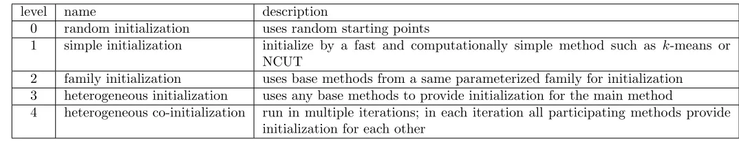
In Table 1, we summarize the above initialization strategies in a hierarchy. 229
The computational cost increases along the hierarchy from low to high levels. 230
We argue that the increased expense is often deserved for improving clustering 231
quality, which will be justified by experiments in the following section. Note 232
Table 1: Summary of the initialization hierarchy for cluster analysis
level name description
0 random initialization uses random starting points
1 simple initialization initialize by a fast and computationally simple method such as k-means or NCUT
2 family initialization uses base methods from a same parameterized family for initialization 3 heterogeneous initialization uses any base methods to provide initialization for the main method
4 heterogeneous co-initialization run in multiple iterations; in each iteration all participating methods provide initialization for each other
5. Experiments
234
We provide two groups of empirical results to demonstrate that 1) cluster-235
ing performance can often be improved using more comprehensive initializations 236
in the proposed hierarchy and 2) the new method outperforms three existing 237
approaches that aggregate clusterings. All datasets and codes used in the ex-238
periments are available online1.
239
5.1. Data sets
240
We focus on clustering tasks on real-world datasets. Nineteen publicly 241
available datasets have been used in our experiments. They are from various 242
domains, including text documents, astroparticles, face images, handwritten 243
digit/letter images, protein. The sizes of these datasets range from a few hun-244
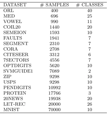
dreds to tens of thousands. The statistics of the datasets are summarized in 245
Table 2. The data sources and descriptions are given in the supplemental doc-246
ument. For fair comparisons, we chose datasets whose ground truth classes are 247
known. 248
The datasets are preprocessed as follows. We first extracted vectorial fea-249
tures for each data sample, in particular, scattering features [30] for images and 250
Tf-Idf features for text documents. In machine learning and data analysis, the 251
vectorial data often lie in a curved manifold, i.e. most simple metrics such as the 252
Euclidean distance or cosine (here for Tf-Idf features) is only reliable in a small 253
1
Table 2: Statistics of the data sets.
DATASET # SAMPLES # CLASSES
ORL 400 40
MED 696 25
VOWEL 990 11
COIL20 1440 20
SEMEION 1593 10
FAULTS 1941 7
SEGMENT 2310 7
CORA 2708 7
CITESEER 3312 6
7SECTORS 4556 7
OPTDIGITS 5620 10
SVMGUIDE1 7089 2
ZIP 9298 10
USPS 9298 10
PENDIGITS 10992 10
PROTEIN 17766 3
20NEWS 19938 20
LET-REC 20000 26
MNIST 70000 10
neighborhood. We employedK-Nearest-Neighbor (KNN) graph to encode such 254
local information. The choice ofK is not very sensitive for large-scale datasets. 255
Here we fix K = 10 for all datasets. We symmetrized the affinity matrix A: 256
Aij = 1 if i is one of theK nearest neighbors ofj, or vice versa, andAij = 0 257
otherwise. 258
5.2. Evaluation criteria
259
The performance of cluster analysis is evaluated by comparing the resulting 260
clusters to ground truth classes. We have adopted two widely used criteria: 261
• purity (e.g. [26, 8]), computed as 262
purity = 1
n r
X
k=1
max
1≤l≤qn l
k, (4)
wherenl
kis the number of vertices in the partitionkthat belong to
ground-263
• normalized mutual information [17], computed as 265
NMI =
Pr i=1
Pr′
j=1ni,jlog
n
i,jn nimj
qPr
i=1nilog
ni n
Pr′
j=1mjlog
mj n
, (5)
whererandr′respectively denote the number of clusters and classes;ni,j
266
is the number of data points agreed by cluster i and class j; ni and mj
267
denote the number of data points in clusteriand classjrespectively; and 268
nis the total number of data points in the dataset. 269
For a given partition of the data, all the above measures give a value between 0 270
and 1. A larger value in general indicates a better clustering performance. 271
5.3. Clustering with initializations at different levels
272
In the first group of experiments, we have tested various clustering methods 273
with different initializations in the hierarchy described in Section 4. We focus 274
on the following four levels: random initialization,simple initialization,
hetero-275
geneous initialization, andheterogeneous co-initialization in these experiments, 276
while treatingfamily initialization as a special case ofheterogeneous
initializa-277
tion. These levels of initializations have been applied to six clustering methods, 278
which are 279
• Projective NMF (PNMF) [31, 32, 28], 280
• Nonnegative Spectral Clustering (NSC) [24], 281
• Symmetric Tri-Factor Orthogonal NMF (ONMF) [26], 282
• Probabilistic Latent Semantic Indexing (PLSI) [33], 283
• Left-Stochastic Matrix Decomposition (LSD) [25], 284
• Data-Cluster-Data random walks (DCD) [8]. 285
For comparison, we also include the results of two other methods based on graph 286
• Normalized Cut (NCUT) [9], 288
• 1-Spectral Ratio Cheeger Cut (1-SPEC) [34]. 289
We have coded NSC, PNMF, ONMF, LSD, DCD, and PLSI using multiplicative 290
updates and ran each of these programs for 10,000 iterations to ensure their 291
convergence. Symmetric versions of PNMF and PLSI have been used. We 292
adopted the 1-SPEC software by Hein and B¨uhler2 with its default setting.
293
Following Yang and Oja [8], we employed four different Dirichlet priors (α = 294
1,1.2,2,5) for DCD, where each with a different prior is treated as a different 295
method inheterogeneous initialization andheterogeneous co-initialization. 296
Forrandom initialization, we ran the clustering methods with fifty starting 297
points, each with a different random seed, and then record the result with the 298
best objective. Forsimple initialization, we employed NCUT to provide initial-299
ization for the six non-graph-cut methods. Precisely, their starting (relaxed) 300
indicator matrix is given by the NCUT result plus 0.2. This same scheme is 301
used in heterogeneous initialization and heterogeneous co-initialization where 302
one method is initialized by another. For heterogeneous co-initialization, the 303
number of co-initialization iterations was set to 5, as in practice we found that 304
there is no significant improvement after five rounds. For any initialization 305
and clustering method, the learned result gives an objective no worse than the 306
initialization. 307
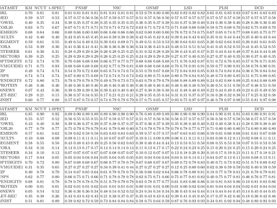
Table 3 shows the clustering performance comparison. For clarity, only the 308
DCD results usingα= 1, i.e., with a uniform prior, are listed in the table, while 309
the complete clustering results including three other Dirichlet priors are given 310
in the supplemental document. 311
There are two types of methods: NCUT and 1-SPEC are of the first type and 312
they are insensitive to starting points, though their results are often mediocre 313
when compared to the best in each row, especially for large datasets. The second 314
type of methods include the other six methods, whose performance depends on 315
2
initializations. Their results are given in cells with quadruples. We can see that 316
more comprehensive initialization strategies often lead to better clusterings, 317
where the four numbers in most cells monotonically increase from left to right. 318
In particular, improvement brought by co-initializations is more often and 319
significant for PLSI and DCD. For example, Table 3 (top) shows that DCD 320
forUSPSdataset, the purity ofheterogeneous co-initialization is 5% better than 321
heterogeneous initialization, 10% better thansimple initialization, and 34% bet-322
ter thanrandom initialization. The advantage of co-initialization for PLSI and 323
DCD is because these two methods are based on Kullback-Leibler (KL-) di-324
vergence. This divergence is more suitable for sparse input similarities due to 325
curved manifolds [8]. However, the objective using KL-divergence involves a 326
more sophisticated surface and is thus difficult to optimize. Therefore these 327
methods require more considerate initializations that provide a good starting 328
point. In contrast, objectives of PNMF, NSC, ONMF and LSD, are relatively 329
easier to optimize. These methods often perform better than PLSI and DCD 330
using lower levels of initializations. However, more comprehensive initializations 331
may not improve their clusterings (see e.g. ONMF forOPTDIGITS). This can be 332
explained by their improper modeling of sparse input similarities based on the 333
Euclidean distance such that more probably a better objective of these methods 334
may not correspond to better clustering performance. 335
The improvement pattern becomes clearer when the dataset is larger. Es-336
pecially, PLSI and DCD achieve remarkable 0.98 purity for the largest dataset 337
MNIST. Note that purity corresponds to classification accuracy up to permuta-338
tion between clusters and classes. This means that our unsupervised cluster 339
analysis results are already very close to state-of-the-art supervised classifica-340
tion results3. A similar purity was reported in DCD using
family initialization. 341
Our experiments show that it is also achievable for other clustering methods 342
given co-initializations, with even better results by PLSI and DCD. 343
3
5.4. Comparison with ensemble clustering
344
Our approach uses a set of clustering methods and outputs a final partition 345
of data samples. There exists another way to combine clustering algorithms: 346
ensemble clustering, which was reviewed in Section 3 . Therefore, we have com-347
pared our co-initialization method with three ensemble clustering methods in the 348
second group of experiments: the BEST algorithm [18], the co-association algo-349
rithm (CO) [19], and the link-based algorithm (CTS) [20]. We coded the BEST 350
and CO algorithms by ourselves and ran the CTS algorithm using LinkCluE 351
package [21]. For fair comparison, the set of base methods (i.e. same objective 352
and same optimization algorithm) is the same for all compared approaches: the 353
11 bases are from NCUT, 1-SPEC, PNMF, NSC, ONMF, LSD, PLSI, DCD1, 354
DCD1.2, DCD2, and DCD5 respectively. The data input for a particular base 355
method is also exactly the same across different combining approaches. The 356
final partitions for CO and CTS were given by the complete-linkage hierarchical 357
clustering algorithm provided in [21]. 358
Different from the other compared approaches, our method actually does not 359
average the clusterings. Each participating clustering method in co-initializations 360
gives their own results, according to the heterogeneous-co-initialization pseu-361
docode in Algorithm 2. Here we chose the result by DCD for the comparison 362
with the ensemble methods, as we find that this method benefits the most from 363
co-initializations. 364
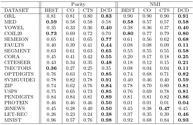
The comparison results are shown in Table 4. We can see that DCD wins 365
most clustering tasks, where it achieves the best for 16 out of 19 datasets in 366
terms of purity, and 18 out of 19 in terms of NMI. The superiority of DCD 367
using co-initializations is especially distinct for large datasets. DCD clearly 368
wins for all but the smallest datasets. 369
6. Conclusions
370
We have presented a new method for improving clustering performance 371
ing scheme that seeks consensus as clustering, our method tries to find better 373
starting points for the participating methods through their initializations for 374
each other. The initialization strategies can be organized in a hierarchy from 375
simple to complex. By extensive experiments on real-world datasets, we have 376
shown that 1) higher-level initialization strategies in the hierarchy can often 377
lead to better clustering performance and 2) the co-initialization method can 378
significantly outperform conventional ensemble clustering methods that average 379
input clusterings. 380
Our findings reflect the importance of pre-training in cluster analysis. There 381
could be more future steps towards this direction. Currently the participat-382
ing methods are chosen heuristically. A more rigorous and computable diver-383
sity measure between clustering methods could be helpful for more efficient 384
co-initializations. A meta probabilistic clustering framework might be also ad-385
vantageous, where the starting points are sampled from more informative priors 386
instead of the uniform distribution. 387
The proposed co-initialization strategy shares similarities with evolutionary 388
algorithms (EA) or genetic algorithms (GA) that use different starting points 389
and combine them to make new solution [35, 36]. In the future work, it would be 390
interesting to find more precise connection between our approach with EA/GA, 391
which could in turn generalize co-initializations to a more powerful framework. 392
References
393
[1] P. Bradley, U. Fayyad, Refining initial points for k-means clustering, in: 394
International Conference on Machine Learning (ICML), 1998, pp. 91–99. 395
[2] A. Likas, N. Vlassis, J. J Verbeek, The global k-means clustering algorithm, 396
Pattern Recognition 36 (2) (2003) 451–461. 397
[3] S. Khan, A. Ahmad, Cluster center initialization algorithm for k-means 398
[4] M. Erisoglu, N. Calis, S. Sakallioglu, A new algorithm for initial cluster 400
centers in k-means algorithm, Pattern Recognition Letters 32 (14) (2011) 401
1701–1705. 402
[5] Z. Zheng, J. Yang, Y. Zhu, Initialization enhancer for non-negative ma-403
trix factorization, Engineering Applications of Artificial Intelligence 20 (1) 404
(2007) 101–110. 405
[6] Y. Kim, S. Choi, A method of initialization for nonnegative matrix fac-406
torization, in: IEEE International Conference on Acoustics, Speech, and 407
Signal Processing (ICASSP), 2007, pp. 537–540. 408
[7] T. Hofmann, Probabilistic latent semantic indexing, in: International Con-409
ference on Research and Development in Information Retrieval (SIGIR), 410
1999, pp. 50–57. 411
[8] Z. Yang, E. Oja, Clustering by low-rank doubly stochastic matrix decom-412
position, in: International Conference on Machine Learning (ICML), 2012, 413
pp. 831–838. 414
[9] J. Shi, J. Malik, Normalized cuts and image segmentation, IEEE Transac-415
tions on Pattern Analysis and Machine Intelligence 22 (8) (2000) 888–905. 416
[10] P. Arbelaez, M. Maire, C. Fowlkes, J. Malik, Contour detection and hier-417
archical image segmentation, IEEE Transactions on Pattern Analysis Ma-418
chine Intelligence 33 (5) (2011) 898–916. 419
[11] Z. Yang, T. Hao, O. Dikmen, X. Chen, E. Oja, Clustering by nonnegative 420
matrix factorization using graph random walk, in: Advances in Neural 421
Information Processing Systems (NIPS), 2012, pp. 1088–1096. 422
[12] D. R. Hunter, K. Lange, A tutorial on MM algorithms, The American 423
Statistician 58 (1) (2004) 30–37. 424
[13] Z. Yang, E. Oja, Unified development of multiplicative algorithms for lin-425
ear and quadratic nonnegative matrix factorization, IEEE Transactions on 426
[14] Z. Yang, E. Oja, Quadratic nonnegative matrix factorization, Pattern 428
Recognition 45 (4) (2012) 1500–1510. 429
[15] Z. Zhu, Z. Yang, E. Oja, Multiplicative updates for learning with stochas-430
tic matrices, in: The 18th conference Scandinavian Conferences on Image 431
Analysis (SCIA), 2013, pp. 143–152. 432
[16] E. Alpaydin, Introduction to Machine Learning, The MIT Press, 2010. 433
[17] A. Strehl, J. Ghosh, Cluster ensembles—a knowledge reuse framework for 434
combining multiple partitions, Journal of Machine Learning Research 3 435
(2003) 583–617. 436
[18] A. Gionis, H. Mannila, P. Tsaparas, Clustering aggregation, in: Interna-437
tional Conference on Data Engineering (ICDE), IEEE, 2005, pp. 341–352. 438
[19] A. Fred, A. Jain, Combining multiple clusterings using evidence accumu-439
lation, IEEE Transactions on Pattern Analysis and Machine Intelligence 440
27 (6) (2005) 835–850. 441
[20] N. Iam-On, T. Boongoen, S. Garrett, Refining pairwise similarity matrix 442
for cluster ensemble problem with cluster relations, in: International Con-443
ference on Discovery Science (DS), Springer, 2008, pp. 222–233. 444
[21] N. Iam-On, S. Garrett, Linkclue: A matlab package for link-based cluster 445
ensembles, Journal of Statistical Software 36 (9) (2010) 1–36. 446
[22] S. Rota Bul`o, A. Louren¸co, A. Fred, M. Pelillo, Pairwise probabilistic clus-447
tering using evidence accumulation, in: International Workshop on Statis-448
tical Techniques in Pattern Recognition (SPR), 2010, pp. 395–404. 449
[23] A. Louren¸co, S. Rota Bul`o, N. Rebagliati, A. Fred, M. Figueiredo, 450
M. Pelillo, Probabilistic consensus clustering using evidence accumulation, 451
Machine Learning, in press (2013). 452
[24] C. Ding, T. Li, M. Jordan, Nonnegative matrix factorization for combinato-453
in: IEEE International Conference on Data Mining (ICDM), IEEE, 2008, 455
pp. 183–192. 456
[25] R. Arora, M. Gupta, A. Kapila, M. Fazel, Clustering by left-stochastic 457
matrix factorization, in: International Conference on Machine Learning 458
(ICML), 2011, pp. 761–768. 459
[26] C. Ding, T. Li, W. Peng, H. Park, Orthogonal nonnegative matrix t-460
factorizations for clustering, in: International Conference on Knowledge 461
Discovery and Data Mining (SIGKDD), ACM, 2006, pp. 126–135. 462
[27] S. Lloyd, Last square quantization in pcm, IEEE Transactions on Informa-463
tion Theory, special issue on quantization 28 (1982) 129–137. 464
[28] Z. Yang, E. Oja, Linear and nonlinear projective nonnegative matrix fac-465
torization, IEEE Transactions on Neural Networks 21 (5) (2010) 734–749. 466
[29] C. Ding, T. Li, W. Peng, On the equivalence between non-negative matrix 467
factorization and probabilistic latent semantic indexing, Computational 468
Statistics & Data Analysis 52 (8) (2008) 3913–3927. 469
[30] S. Mallat, Group invariant scattering, Communications on Pure and Ap-470
plied Mathematics 65 (10) (2012) 1331–1398. 471
[31] Z. Yuan, E. Oja, Projective nonnegative matrix factorization for image 472
compression and feature extraction, in: Proceedings of 14th Scandinavian 473
Conference on Image Analysis (SCIA), Joensuu, Finland, 2005, pp. 333– 474
342. 475
[32] Z. Yang, Z. Yuan, J. Laaksonen, Projective non-negative matrix factoriza-476
tion with applications to facial image processing, International Journal on 477
Pattern Recognition and Artificial Intelligence 21 (8) (2007) 1353–1362. 478
[33] T. Hofmann, Probabilistic latent semantic indexing, in: International Con-479
ference on Research and Development in Information Retrieval (SIGIR), 480
[34] M. Hein, T. B¨uhler, An inverse power method for nonlinear eigenproblems 482
with applications in 1-Spectral clustering and sparse PCA, in: Advances in 483
Neural Information Processing Systems (NIPS), 2010, pp. 847–855. 484
[35] E. R. Hruschka, R. J. G. B. Campello, A. A. Freitas, A. P. L. F. De Car-485
valho, A survey of evolutionary algorithms for clustering, IEEE Transac-486
tions on Systems, Man, and Cybernetics, Part C: Applications and Reviews 487
39 (2) (2009) 133–155. 488
[36] M. J. Abul Hasan, S. Ramakrishnan, A survey: hybrid evolutionary al-489
gorithms for cluster analysis, Artificial Intelligence Review 36 (3) (2011) 490
Table 3: Clustering performance of various clustering methods with different initializations. Performances are measured by (top) Purity and (bottom) NMI. Rows are ordered by dataset sizes. In cells with quadruples, the four numbers from left to right are results usingrandom,simple, andheterogeneous initializa-tionandheterogeneous co-initialization.
DATASET KM NCUT 1-SPEC PNMF NSC ONMF LSD PLSI DCD
ORL 0.70 0.81 0.81 0.81 0.81 0.81 0.81 0.81 0.81 0.81 0.81 0.53 0.78 0.80 0.80 0.82 0.82 0.82 0.82 0.65 0.81 0.83 0.83 0.67 0.81 0.83 0.83 MED 0.59 0.57 0.53 0.57 0.57 0.56 0.56 0.57 0.59 0.57 0.57 0.51 0.57 0.56 0.56 0.57 0.57 0.57 0.57 0.57 0.57 0.57 0.58 0.57 0.57 0.57 0.58 VOWEL 0.40 0.35 0.34 0.38 0.35 0.37 0.38 0.35 0.35 0.35 0.35 0.36 0.35 0.37 0.38 0.34 0.37 0.38 0.40 0.34 0.36 0.38 0.40 0.28 0.36 0.36 0.40 COIL20 0.63 0.71 0.67 0.67 0.71 0.71 0.71 0.73 0.71 0.72 0.72 0.63 0.71 0.72 0.72 0.71 0.68 0.68 0.68 0.58 0.75 0.69 0.70 0.62 0.75 0.69 0.70 SEMEION 0.68 0.64 0.66 0.60 0.66 0.60 0.60 0.66 0.66 0.66 0.66 0.62 0.60 0.60 0.60 0.76 0.72 0.74 0.75 0.67 0.65 0.74 0.77 0.68 0.65 0.75 0.77 FAULTS 0.42 0.40 0.40 0.42 0.45 0.45 0.45 0.44 0.39 0.38 0.38 0.42 0.45 0.42 0.42 0.39 0.44 0.43 0.43 0.35 0.41 0.44 0.44 0.35 0.40 0.43 0.44 SEGMENT 0.59 0.61 0.55 0.49 0.54 0.49 0.53 0.39 0.61 0.69 0.71 0.49 0.51 0.53 0.53 0.30 0.64 0.61 0.65 0.26 0.62 0.64 0.65 0.26 0.61 0.61 0.65 CORA 0.53 0.39 0.36 0.41 0.36 0.41 0.41 0.36 0.36 0.36 0.36 0.34 0.36 0.43 0.43 0.48 0.51 0.51 0.54 0.41 0.45 0.52 0.55 0.41 0.45 0.52 0.55 CITESEER 0.61 0.30 0.31 0.28 0.29 0.29 0.28 0.26 0.28 0.25 0.25 0.31 0.32 0.28 0.28 0.38 0.43 0.45 0.47 0.35 0.44 0.44 0.48 0.37 0.44 0.44 0.48 7SECTORS 0.39 0.25 0.25 0.29 0.29 0.29 0.29 0.26 0.25 0.25 0.25 0.24 0.29 0.29 0.29 0.27 0.37 0.40 0.35 0.27 0.37 0.40 0.35 0.30 0.37 0.40 0.35 OPTDIGITS 0.72 0.74 0.76 0.70 0.68 0.68 0.68 0.66 0.77 0.77 0.77 0.68 0.68 0.68 0.68 0.71 0.76 0.82 0.87 0.51 0.72 0.76 0.85 0.57 0.76 0.71 0.85 SVMGUIDE1 0.71 0.75 0.93 0.68 0.68 0.68 0.68 0.82 0.77 0.79 0.81 0.68 0.68 0.68 0.68 0.70 0.78 0.91 0.91 0.59 0.77 0.90 0.91 0.58 0.78 0.90 0.91 ZIP 0.49 0.74 0.74 0.54 0.70 0.72 0.68 0.65 0.74 0.74 0.74 0.55 0.70 0.67 0.68 0.72 0.84 0.83 0.85 0.33 0.74 0.84 0.84 0.36 0.76 0.84 0.84 USPS 0.74 0.74 0.74 0.67 0.80 0.75 0.68 0.72 0.74 0.74 0.74 0.62 0.80 0.75 0.68 0.80 0.79 0.84 0.85 0.48 0.73 0.80 0.85 0.51 0.75 0.80 0.85 PENDIGITS 0.72 0.80 0.73 0.79 0.79 0.79 0.79 0.49 0.79 0.73 0.73 0.63 0.79 0.79 0.79 0.66 0.88 0.89 0.89 0.24 0.82 0.88 0.89 0.25 0.84 0.88 0.89 PROTEIN 0.46 0.46 0.46 0.46 0.46 0.46 0.46 0.46 0.46 0.46 0.46 0.46 0.46 0.46 0.46 0.46 0.46 0.48 0.50 0.46 0.51 0.51 0.50 0.47 0.46 0.51 0.50 20NEWS 0.07 0.43 0.36 0.39 0.39 0.39 0.38 0.39 0.43 0.40 0.40 0.27 0.38 0.38 0.38 0.41 0.48 0.48 0.49 0.22 0.44 0.49 0.49 0.23 0.45 0.49 0.50 LET-REC 0.29 0.21 0.15 0.36 0.37 0.34 0.35 0.17 0.21 0.21 0.21 0.29 0.35 0.35 0.34 0.31 0.31 0.37 0.37 0.16 0.26 0.32 0.38 0.17 0.25 0.32 0.38 MNIST 0.60 0.77 0.88 0.57 0.87 0.73 0.57 0.74 0.79 0.79 0.79 0.57 0.75 0.65 0.57 0.93 0.75 0.97 0.97 0.46 0.79 0.97 0.98 0.55 0.81 0.97 0.98
DATASET KM NCUT 1-SPEC PNMF NSC ONMF LSD PLSI DCD
Table 4: Clustering performance comparison of DCD using heterogeneous co-initialization with three ensemble clustering methods. Rows are ordered by dataset sizes. Boldface numbers indicate the best. The 11 bases are from NCUT, 1-SPEC, PNMF, NSC, ONMF, LSD, PLSI, DCD1, DCD1.2, DCD2, and DCD5 respectively.
Purity NMI
DATASET BEST CO CTS DCD BEST CO CTS DCD
ORL 0.81 0.81 0.80 0.83 0.90 0.90 0.90 0.91
MED 0.59 0.58 0.58 0.58 0.58 0.57 0.57 0.58
VOWEL 0.35 0.33 0.36 0.40 0.38 0.36 0.37 0.40
COIL20 0.73 0.69 0.72 0.70 0.80 0.77 0.79 0.80
SEMEION 0.65 0.61 0.65 0.77 0.61 0.56 0.62 0.68
FAULTS 0.40 0.39 0.41 0.44 0.08 0.08 0.09 0.11
SEGMENT 0.63 0.61 0.63 0.65 0.55 0.55 0.55 0.58
CORA 0.45 0.41 0.42 0.55 0.20 0.17 0.18 0.25
CITESEER 0.43 0.34 0.35 0.48 0.18 0.12 0.15 0.21
7SECTORS 0.36 0.27 0.25 0.35 0.08 0.04 0.04 0.11
OPTDIGITS 0.76 0.63 0.71 0.85 0.74 0.68 0.71 0.82
SVMGUIDE1 0.78 0.82 0.78 0.91 0.40 0.46 0.40 0.59
ZIP 0.74 0.62 0.76 0.84 0.78 0.70 0.80 0.81
USPS 0.75 0.65 0.73 0.85 0.76 0.69 0.78 0.81
PENDIGITS 0.84 0.84 0.81 0.89 0.81 0.81 0.82 0.86
PROTEIN 0.46 0.46 0.46 0.50 0.01 0.01 0.01 0.04
20NEWS 0.45 0.28 0.40 0.50 0.45 0.38 0.47 0.45
LET-REC 0.26 0.23 0.24 0.38 0.37 0.35 0.39 0.46