Precalculus wih Limites free download

(1)

(2)

GRAPHS OF PARENT FUNCTIONS

Linear Function Absolute Value Function Square Root Function

Domain: Domain: Domain:

Range: Range: Range:

x-intercept: Intercept: Intercept:

y-intercept: Decreasing on Increasing on

Increasing when Increasing on

Decreasing when Even function

y-axis symmetry

Greatest Integer Function Quadratic (Squaring) Function Cubic Function

Range: the set of integers Range : Range:

x-intercepts: in the interval Range : Intercept:

y-intercept: Intercept: Increasing on

Constant between each pair of Decreasing on for Odd function

consecutive integers Increasing on for Origin symmetry

Jumps vertically one unit at Increasing on for

each integer value Decreasing on for

Even function y-axis symmetry Relative minimum

relative maximum or vertex:0, 0

a < 0, a > 0,

a< 0 0,

_⬁

a < 0 ⫺

_⬁

, 0

a> 0 0,

_⬁

a > 0 ⫺

_⬁

, 0

⫺

_⬁

,

_⬁

0, 0

0, 0 ⫺

_⬁

, 0

a < 0 0, 1

⫺

_⬁

,

_⬁

0,

_⬁

a> 0

⫺

_⬁

,

_⬁

⫺

_⬁

,

_⬁

⫺

_⬁

,

_⬁

x y

(0, 0)

f(x)=x3

−2

−3 1 2 3

−2

−1

−3 2 3

x y

−1

−2 1 2 3 4 1

−1

−2

−3 2 3

f(x) =ax2,a>0

f(x) =ax2,a<0 x

y

1

−1

−2

−3 2 3

−3 1 2 3

f(x) =[[ ]]x

fx⫽x3 fx⫽ax2

fx⫽x

m < 0

0,

_⬁

m > 0

0,

_⬁

⫺

_⬁

, 0

0,b

0, 0 0, 0

⫺bm, 0

0,

_⬁

0,

_⬁

⫺

_⬁

,

_⬁

0,

_⬁

⫺

_⬁

,

_⬁

⫺

_⬁

,

_⬁

x y

−1 2 3 4

−1 1 2 3 4

(0, 0)

f(x) = x

x y

−1

−2 2

−1

−2 1 2

(0, 0)

f(x) = x_

x y

(0,b)

b m

(

− , 0

(

− , 0_mb

(

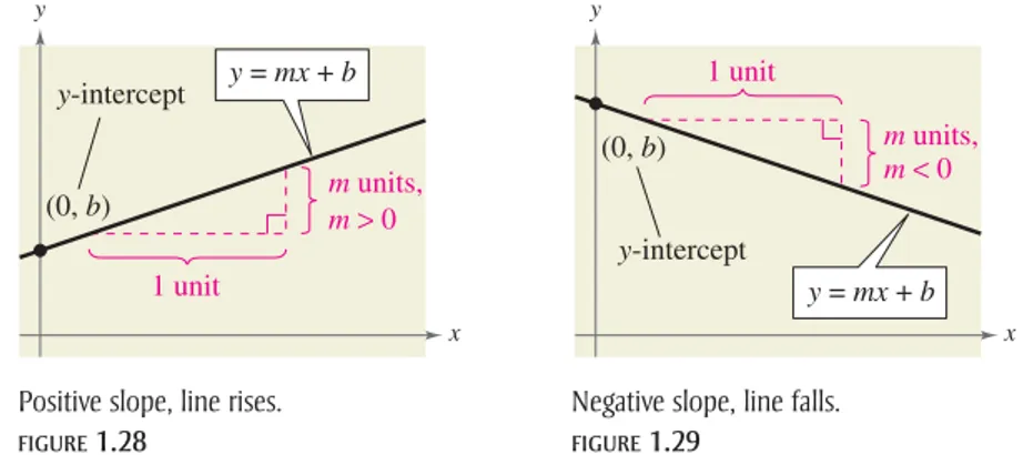
f(x) = mx + b,

m > 0

f(x) = mx + b,

m < 0

fx⫽ x

fx⫽

x

⫽

x, ⫺x,

(3)

Rational (Reciprocal) Function Exponential Function Logarithmic Function

Range: Range: Range:

No intercepts Intercept: Intercept:

Decreasing on and Increasing on Increasing on

Odd function for Vertical asymptote:y-axis

Origin symmetry Decreasing on Continuous

Vertical asymptote:y-axis for Reflection of graph of

Horizontal asymptote:x-axis Horizontal asymptote:x-axis in the line Continuous

Sine Function Cosine Function Tangent Function

Domain: all Range: Period: x-intercepts: y-intercept:

Vertical asymptotes:

Odd function Origin symmetry

x⫽ ␲ 2⫹n␲

0, 0 n␲, 0 ␲

⫺

_⬁

,

_⬁

x⫽ ␲

2⫹n␲

2

1 3

π π

2

π

2

−

f(x) = tan x

x y

3π 2

−2

−3 2 3

π π π

2

π π

2

− ₋

f(x) = cos x

x

2

y

1

−2

−3 2 3

π π π

2

π −

f(x) = sin x

x

2

y

fx⫽tanx fx⫽cosx

fx⫽sinx

y⫽x

fx⫽ax

fx⫽a⫺x

⫺

_⬁

,

_⬁

fx⫽ax

0,

_⬁

⫺

_⬁

,

_⬁

0,

_⬁

⫺

_⬁

, 0

1, 0 0, 1

⫺

_⬁

,

_⬁

0,

_⬁

⫺

_⬁

, 0傼0,

_⬁

)

0,

_⬁

⫺

_⬁

,

_⬁

⫺

_⬁

, 0傼0,

_⬁

)

x y

f(x) = log_a x

1 2

−1 1

(1, 0)

x y

(0, 1)

f(x)=a−x f(x)=ax

x y

f(x) = 1

x

−1 1 2 3 1

2 3

fx⫽log_ax, a > 0, a⫽1 fx⫽ax_, _a> 0, a⫽1

fx⫽1 x

Domain: Range: Period: x-intercepts: y-intercept: Odd function Origin symmetry

0, 0 n␲, 0 2␲

⫺1, 1

⫺

_⬁

,

_⬁

Domain:

Range: Period: x-intercepts: y-intercept: Even function y-axis symmetry

0, 1

␲

2 ⫹n␲, 0

2␲

(4)

Cosecant Function Secant Function Cotangent Function

Domain: all Range:

Inverse Sine Function Inverse Cosine Function Inverse Tangent Function

Domain:

Domain: all Range: Period: y-intercept:

Vertical asymptotes:

Even function y-axis symmetry

(5)

Precalculus with Limits

Second Edition

Ron Larson

The Pennsylvania State University

The Behrend College

With the assistance of

David C. Falvo

The Pennsylvania State University

The Behrend College

(6)

Precalculus with Limits, Second Edition

Ron Larson

Publisher: Charlie VanWagner

Acquiring Sponsoring Editor: Gary Whalen Development Editor: Stacy Green Assistant Editor: Cynthia Ashton Editorial Assistant: Guanglei Zhang Associate Media Editor: Lynh Pham Marketing Manager: Myriah FitzGibbon Marketing Coordinator: Angela Kim

Marketing Communications Manager: Katy Malatesta Content Project Manager: Susan Miscio

Senior Art Director: Jill Ort Senior Print Buyer: Diane Gibbons Production Editor: Carol Merrigan Text Designer: Walter Kopek

Rights Acquiring Account Manager, Photos: Don Schlotman Photo Researcher: Prepress PMG

Cover Designer: Harold Burch

Cover Image: Richard Edelman/Woodstock Graphics Studio Compositor: Larson Texts, Inc.

ALL RIGHTS RESERVED. No part of this work covered by the copyright herein may be reproduced, transmitted, stored, or used in any form or by any means graphic, electronic, or mechanical, including but not limited to photocopying, recording, scanning, digitizing, taping, Web distribution, information networks, or information storage and retrieval systems, except as permitted under Section 107 or 108 of the 1976 United States Copyright Act, without the prior written permission of the publisher.

Brooks/Cole

10 Davis Drive

Belmont, CA 94002-3098 USA

Cengage Learning is a leading provider of customized learning solutions with office locations around the globe, including Singapore, the United Kingdom, Australia, Mexico, Brazil, and Japan. Locate your local office at:

international.cengage.com/region

Cengage Learning products are represented in Canada by Nelson Education, Ltd.

For your course and learning solutions, visit www.cengage.com

Purchase any of our products at your local college store or at our preferred online store www.ichapters.com

For product information and technology assistance, contact us at

Cengage Learning Customer & Sales Support, 1-800-354-9706

For permission to use material from this text or product, submit all requests online at www.cengage.com/permissions.

Further permissions questions can be emailed to

permissionrequest@cengage.com

Printed in the United States of America 1 2 3 4 5 6 7 13 12 11 10 09

Library of Congress Control Number: 2009930251 Student Edition:

(7)

iii

A Word from the Author (Preface) vii

Functions and Their Graphs

1

1.1 Rectangular Coordinates 2

1.2 Graphs of Equations 13

1.3 Linear Equations in Two Variables 24

1.4 Functions 39

1.5 Analyzing Graphs of Functions 54

1.6 A Library of Parent Functions 66

1.7 Transformations of Functions 73

1.8 Combinations of Functions: Composite Functions 83

1.9 Inverse Functions 92

1.10 Mathematical Modeling and Variation 102

Chapter Summary 114 Review Exercises 116 Chapter Test 121 Proofs in Mathematics 122 Problem Solving 123

Polynomial and Rational Functions

125

2.1 Quadratic Functions and Models 126

2.2 Polynomial Functions of Higher Degree 136

2.3 Polynomial and Synthetic Division 150

2.4 Complex Numbers 159

2.5 Zeros of Polynomial Functions 166

2.6 Rational Functions 181

2.7 Nonlinear Inequalities 194

Exponential and Logarithmic Functions

215

3.1 Exponential Functions and Their Graphs 216

3.2 Logarithmic Functions and Their Graphs 227

3.3 Properties of Logarithms 237

3.4 Exponential and Logarithmic Equations 244

3.5 Exponential and Logarithmic Models 255

Chapter Summary 268 Review Exercises 270

Chapter Test 273 Cumulative Test for Chapters 1–3 274 Proofs in Mathematics 276 Problem Solving 277

chapter

1 chapter

2

(8)

iv Contents

Trigonometry

279

4.1 Radian and Degree Measure 280

4.2 Trigonometric Functions: The Unit Circle 292

4.3 Right Triangle Trigonometry 299

4.4 Trigonometric Functions of Any Angle 310

4.5 Graphs of Sine and Cosine Functions 319

4.6 Graphs of Other Trigonometric Functions 330

4.7 Inverse Trigonometric Functions 341

4.8 Applications and Models 351

Analytic Trigonometry

371

5.1 Using Fundamental Identities 372

5.2 Verifying Trigonometric Identities 380

5.3 Solving Trigonometric Equations 387

5.4 Sum and Difference Formulas 398

5.5 Multiple-Angle and Product-to-Sum Formulas 405 Chapter Summary 416 Review Exercises 418 Chapter Test 421 Proofs in Mathematics 422 Problem Solving 425

Additional Topics in Trigonometry

427

6.1 Law of Sines 428

6.2 Law of Cosines 437

6.3 Vectors in the Plane 445

6.4 Vectors and Dot Products 458

6.5 Trigonometric Form of a Complex Number 468 Chapter Summary 478 Review Exercises 480

Systems of Equations and Inequalities

493

7.1 Linear and Nonlinear Systems of Equations 494

7.2 Two-Variable Linear Systems 505

7.3 Multivariable Linear Systems 517

7.4 Partial Fractions 530

7.5 Systems of Inequalities 538

chapter

4 chapter

5 chapter

6

(9)

Contents v

7.6 Linear Programming 549

Matrices and Determinants

569

8.1 Matrices and Systems of Equations 570

8.2 Operations with Matrices 584

8.3 The Inverse of a Square Matrix 599

8.4 The Determinant of a Square Matrix 608

8.5 Applications of Matrices and Determinants 616 Chapter Summary 628 Review Exercises 630 Chapter Test 635 Proofs in Mathematics 636 Problem Solving 637

Sequences, Series, and Probability

639

9.1 Sequences and Series 640

9.2 Arithmetic Sequences and Partial Sums 651

9.3 Geometric Sequences and Series 661

9.4 Mathematical Induction 671

9.5 The Binomial Theorem 681

9.6 Counting Principles 689

9.7 Probability 699

Topics in Analytic Geometry

725

10.1 Lines 726

10.2 Introduction to Conics: Parabolas 733

10.3 Ellipses 742

10.4 Hyperbolas 751

10.5 Rotation of Conics 761

10.6 Parametric Equations 769

10.7 Polar Coordinates 777

10.8 Graphs of Polar Equations 783

10.9 Polar Equations of Conics 791

chapter

8 chapter

9

(10)

vi Contents

chapter

11 chapter

12 Analytic Geometry in Three Dimensions

809

11.1 The Three-Dimensional Coordinate System 810

11.2 Vectors in Space 817

11.3 The Cross Product of Two Vectors 824

11.4 Lines and Planes in Space 831

Limits and an Introduction to Calculus

849

12.1 Introduction to Limits 850

12.2 Techniques for Evaluating Limits 861

12.3 The Tangent Line Problem 871

12.4 Limits at Infinity and Limits of Sequences 881

12.5 The Area Problem 890

Appendix A Review of Fundamental Concepts of Algebra

A1

A.1 Real Numbers and Their Properties A1

A.2 Exponents and Radicals A14

A.3 Polynomials and Factoring A27

A.4 Rational Expressions A39

A.5 Solving Equations A49

A.6 Linear Inequalities in One Variable A63

A.7 Errors and the Algebra of Calculus A73

Answers to Odd-Numbered Exercises and Tests

A81

Index

A211

Index of Applications (web)

Appendix B Concepts in Statistics (web)

B.1 Representing Data

B.2 Measures of Central Tendency and Dispersion

(11)

vii

In this edition, we continue to offer instructors and students a text that is pedagogically sound, mathematically precise, and still comprehensible. There are many changes in the mathematics, art, and design; the more significant changes are noted here.

• New Chapter Openers EachChapter Openerhas three parts, In Mathematics, In

Real Life, and In Careers. In Mathematics describes an important mathematical

topic taught in the chapter. In Real Lifetells students where they will encounter this topic in real-life situations. In Careersrelates application exercises to a variety of careers.

• New Study Tips and Warning/Cautions Insightful information is given to students in two new features. The Study Tip provides students with useful information or suggestions for learning the topic. The Warning/Cautionpoints out common mathematical errors made by students.

• New Algebra Helps Algebra Help directs students to sections of the textbook where they can review algebra skills needed to master the current topic.

• New Side-by-Side Examples Throughout the text, we present solutions to many examples from multiple perspectives—algebraically, graphically, and numerically. The side-by-side format of this pedagogical feature helps students to see that a problem can be solved in more than one way and to see that different methods yield the same result. The side-by-side format also addresses many different learning styles.

A Word from

the Author

Welcome to the Second Edition of Precalculus with Limits! We are proud to offer you a new and revised version of our textbook. With the Second Edition, we have listened to you, our users, and have incorporated many of your suggestions for improvement.

(12)

• New Capstone Exercises Capstonesare conceptual problems that synthesize key topics and provide students with a better understanding of each section’s concepts. Capstone exercises are excellent for classroom discussion or test prep, and teachers may find value in integrating these problems into their reviews of the section.

• New Chapter Summaries The Chapter Summary now includes an explanation and/or example of each objective taught in the chapter.

• Revised Exercise Sets The exercise sets have been carefully and extensively

examined to ensure they are rigorous and cover all topics suggested by our users. Many new skill-building and challenging exercises have been added.

For the past several years, we’ve maintained an independent website—

CalcChat.com—that provides free solutions to all odd-numbered exercises in the text.

Thousands of students using our textbooks have visited the site for practice and help with their homework. For the Second Edition, we were able to use information from CalcChat.com, including which solutions students accessed most often, to help guide the revision of the exercises.

I hope you enjoy the Second Edition of Precalculus with Limits. As always, I welcome comments and suggestions for continued improvements.

(13)

ix

I would like to thank the many people who have helped me prepare the text and the supplements package. Their encouragement, criticisms, and suggestions have been invaluable.

Thank you to all of the instructors who took the time to review the changes in this edition and to provide suggestions for improving it. Without your help, this book would not be possible.

Reviewers

Chad Pierson, University of Minnesota-Duluth; Sally Shao, Cleveland State University; Ed Stumpf, Central Carolina Community College; Fuzhen Zhang, Nova Southeastern

University; Dennis Shepherd, University of Colorado, Denver; Rhonda Kilgo,

Jacksonville State University; C. Altay Özgener, Manatee Community College

Bradenton; William Forrest, Baton Rouge Community College; Tracy Cook, University of Tennessee Knoxville; Charles Hale, California State Poly University Pomona; Samuel Evers, University of Alabama; Seongchun Kwon, University of Toledo; Dr. Arun K. Agarwal, Grambling State University; Hyounkyun Oh, Savannah State University; Michael J. McConnell, Clarion University; Martha Chalhoub, Collin County

Community College; Angela Lee Everett, Chattanooga State Tech Community College;

Heather Van Dyke, Walla Walla Community College; Gregory Buthusiem, Burlington

County Community College; Ward Shaffer, College of Coastal Georgia; Carmen

Thomas,Chatham University; Emily J. Keaton

My thanks to David Falvo, The Behrend College, The Pennsylvania State University, for his contributions to this project. My thanks also to Robert Hostetler, The Behrend College, The Pennsylvania State University, and Bruce Edwards, University of Florida, for their significant contributions to previous editions of this text.

I would also like to thank the staff at Larson Texts, Inc. who assisted with proof-reading the manuscript, preparing and proofproof-reading the art package, and checking and typesetting the supplements.

On a personal level, I am grateful to my spouse, Deanna Gilbert Larson, for her love, patience, and support. Also, a special thanks goes to R. Scott O’Neil. If you have suggestions for improving this text, please feel free to write to me. Over the past two decades I have received many useful comments from both instructors and students, and I value these comments very highly.

Ron Larson

(14)

x

Supplements

Supplements for the Instructor

Annotated Instructor’s Edition This AIE is the complete student text plus point-of-use annotations for the instructor, including extra projects, classroom activities, teaching strategies, and additional examples. Answers to even-numbered text exercises, Vocabulary Checks, and Explorations are also provided.

Complete Solutions Manual This manual contains solutions to all exercises from the text, including Chapter Review Exercises and Chapter Tests.

Instructor’s Companion Website This free companion website contains an abundance of instructor resources.

PowerLecture™with ExamView® The CD-ROM provides the instructor with dynamic media tools for teaching college algebra. PowerPoint® lecture slides and art slides of the figures from the text, together with electronic files for the test bank and a link to the Solution Builder, are available. The algorithmic ExamView allows you to create, deliver, and customize tests (both print and online) in minutes with this easy-to-use assessment system. Enhance how your students interact with you, your lecture, and each other.

Solutions Builder This is an electronic version of the complete solutions manual available via the PowerLecture and Instructor’s Companion Website. It provides instructors with an efficient method for creating solution sets to homework or exams that can then be printed or posted.

(15)

Supplements xi

Supplements for the Student

Student Companion Website This free companion website contains an abundance of student resources.

Instructional DVDs Keyed to the text by section, these DVDs provide comprehensive coverage of the course—along with additional explanations of concepts, sample problems, and applications—to help students review essential topics.

Student Study and Solutions Manual This guide offers step-by-step solutions for all odd-numbered text exercises, Chapter and Cumulative Tests, and Practice Tests with solutions.

Premium eBook The Premium eBook offers an interactive version of the textbook with search features, highlighting and note-making tools, and direct links to videos or tutorials that elaborate on the text discussions.

Enhanced WebAssign Enhanced WebAssign is designed for you to do your homework online. This proven and reliable system uses pedagogy and content found in Larson’s text, and then enhances it to help you learn Precalculus more effectively. Automatically graded homework allows you to focus on your learning and get interactive study assistance outside of class.

(16)

(17)

1

Functions and

Their Graphs

1.1 Rectangular Coordinates

1.2 Graphs of Equations

1.3 Linear Equations in Two Variables

1.4 Functions

1.5 Analyzing Graphs of Functions

1.6 A Library of Parent Functions

1.7 Transformations of Functions

1.9 Inverse Functions

1.8 Combinations of Functions:

1.10 Mathematical Modeling and Variation

Composite Functions

In Mathematics

Functions show how one variable is related to another variable.

In Real Life

Functions are used to estimate values, simulate processes, and discover relation-ships. For instance, you can model the enrollment rate of children in preschool and estimate the year in which the rate will reach a certain number. Such an estimate can be used to plan measures for meeting future needs, such as hiring additional teachers and buying more books. (See Exercise 113, page 64.)

IN CAREERS

There are many careers that use functions. Several are listed below.

Jose Luis Pelaez/Getty Images

• Financial analyst Exercise 95, page 51 • Biologist

Exercise 73, page 91

• Tax preparer

Example 3, page 104 • Oceanographer

Exercise 83, page 112

(18)

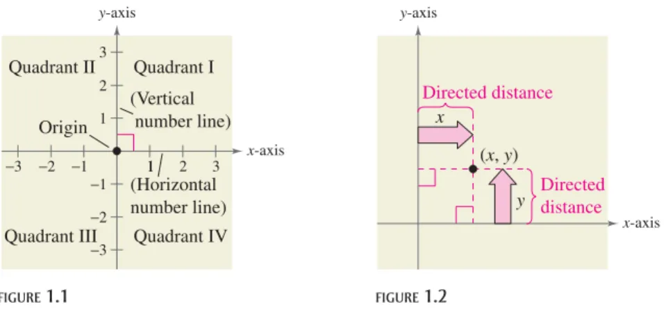
The Cartesian Plane

Just as you can represent real numbers by points on a real number line, you can represent ordered pairs of real numbers by points in a plane called the rectangular coordinate system, or the Cartesian plane, named after the French mathematician René Descartes (1596–1650).

The Cartesian plane is formed by using two real number lines intersecting at right angles, as shown in Figure 1.1. The horizontal real number line is usually called the

x-axis, and the vertical real number line is usually called the y-axis. The point of intersection of these two axes is the origin,and the two axes divide the plane into four parts called quadrants.

FIGURE1.1 FIGURE1.2

Each point in the plane corresponds to an ordered pair of real numbers and calledcoordinatesof the point. The x-coordinaterepresents the directed distance from the -axis to the point, and the y-coordinaterepresents the directed distance from the -axis to the point, as shown in Figure 1.2.

The notation denotes both a point in the plane and an open interval on the real number line. The context will tell you which meaning is intended.

Plotting Points in the Cartesian Plane

Plot the points and

Solution

To plot the point imagine a vertical line through on the -axis and a horizontal line through 2 on the -axis. The intersection of these two lines is the point

The other four points can be plotted in a similar way, as shown in Figure 1.3. Now try Exercise 7.

⫺1, 2.

y

x ⫺1

⫺1, 2,

⫺2,⫺3. ⫺1, 2,3, 4,0, 0,3, 0,

Example 1

x,y

Directed distance fromx-axis x,y

Directed distance fromy-axis x

y y,

x (x,y)

x-axis

(x,y)

x

y

Directed distance

Directed distance y-axis

x-axis

−3 −2 −1 11 2 3 1

2 3

−1

−2

−3

(Vertical number line)

(Horizontal number line)

Quadrant I Quadrant II

Quadrant III Quadrant IV Origin

y-axis

2 Chapter 1 Functions and Their Graphs

1.1 R

ECTANGULAR

C

OORDINATES

What you should learn

• Plot points in the Cartesian plane. • Use the Distance Formula to find

the distance between two points. • Use the Midpoint Formula to find

the midpoint of a line segment. • Use a coordinate plane to model

and solve real-life problems.

Why you should learn it

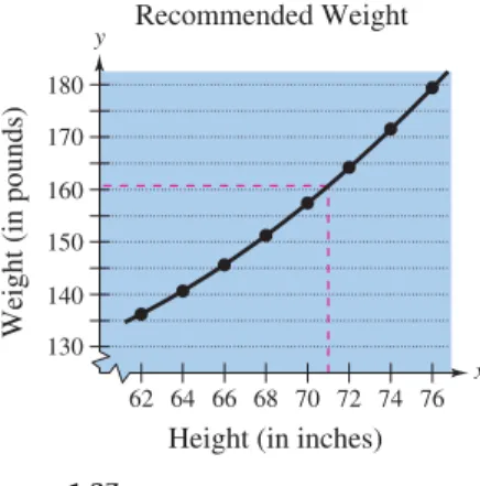
The Cartesian plane can be used to represent relationships between two variables. For instance, in Exercise 70 on page 11, a graph represents the minimum wage in the United States from 1950 to 2009.

1 3 4

−1

−2

−4

(3, 4)

x

−4 −3 −1 1 2 3 4

(3, 0) (0, 0)

( 1, 2)−

( 2, 3)− − y

FIGURE1.3

(19)

Section 1.1 Rectangular Coordinates 3

The beauty of a rectangular coordinate system is that it allows you to see relation-ships between two variables. It would be difficult to overestimate the importance of Descartes’s introduction of coordinates in the plane. Today, his ideas are in common use in virtually every scientific and business-related field.

Sketching a Scatter Plot

From 1994 through 2007, the numbers (in millions) of subscribers to a cellular telecommunication service in the United States are shown in the table, where represents the year. Sketch a scatter plot of the data. (Source: CTIA-The Wireless Association)

Solution

To sketch a scatter plotof the data shown in the table, you simply represent each pair of values by an ordered pair and plot the resulting points, as shown in Figure 1.4. For instance, the first pair of values is represented by the ordered pair

Note that the break in the -axis indicates that the numbers between 0 and 1994 have been omitted.

FIGURE1.4

Now try Exercise 25.

In Example 2, you could have let represent the year 1994. In that case, the horizontal axis would not have been broken, and the tick marks would have been labeled 1 through 14 (instead of 1994 through 2007).

t⫽1 1994 1996 50

100 150 200 250 300

1998 2000 2002 2004 2006

Year

Number of subscribers

(in millions)

Subscribers to a Cellular Telecommunication Service

t N

t

1994, 24.1. t,N

t N

Example 2

T E C H N O LO G Y

The scatter plot in Example 2 is only one way to represent the data graphically. You could also represent the data using a bar graph or a line graph. If you have access to a graphing utility, try using it to represent graphically the data given in Example 2.

Year,t Subscribers,N

1994 1995 1996 1997 1998 1999 2000 2001 2002 2003 2004 2005 2006 2007

(20)

The Pythagorean Theorem and the Distance Formula

The following famous theorem is used extensively throughout this course.

Suppose you want to determine the distance between two points and in the plane. With these two points, a right triangle can be formed, as shown in Figure 1.6. The length of the vertical side of the triangle is and the length of the horizontal side is By the Pythagorean Theorem, you can write

This result is the Distance Formula.

⫽ x2⫺x12⫹y2⫺y12. d⫽

x2⫺x1

2⫹

y2⫺y1

2

d2_⫽

_x

2⫺x1

2⫹

y2⫺y1

2

x2⫺x1

.

y2⫺y1

, x2,y2

x1,y1 d

Pythagorean Theorem

For a right triangle with hypotenuse of length and sides of lengths and you have as shown in Figure 1.5. (The converse is also true. That is, if

then the triangle is a right triangle.) a2_⫹_b2_⫽_c2_,

a2_⫹_b2_⫽_c2_,

b, a c

The Distance Formula

The distance between the points and in the plane is d⫽ x2⫺x12⫹y2⫺y12.

x2,y2 x1,y1

d

Graphical Solution

Use centimeter graph paper to plot the points and Carefully sketch the line segment from to Then use a centimeter ruler to measure the length of the segment.

FIGURE1.7

The line segment measures about 5.8 centimeters, as shown in Figure 1.7. So, the distance between the points is about 5.8 units.

1 2 3 4 5 6 7

cm

B. A B3, 4.

A⫺2, 1 Finding a Distance

Find the distance between the points ⫺2, 1and 3, 4.

Example 3

Algebraic Solution

Let and Then apply the

Distance Formula.

Distance Formula

Simplify.

Use a calculator.

So, the distance between the points is about 5.83 units. You can use the Pythagorean Theorem to check that the distance is correct.

Pythagorean Theorem

Substitute for d.

Distance checks.

✓

Now try Exercise 31. 34⫽34

34

2⫽? 32_⫹₅2 d2_⫽? ₃2_⫹₅2 5.83

⫽ 34

⫽ 52_⫹₃2

⫽ 3⫺⫺22_⫹₄_⫺₁2 d⫽ x2⫺x12⫹y2⫺y12

x2,y2⫽3, 4. x1,y1⫽⫺2, 1

Substitute for x1,y1,x2, and y2. a

b c

a2 + b2 = c2

FIGURE1.5

x

x₁ x₂

x₂− x₁ y₂− y₁

y 1

y 2

d

(x₁, y₂) (x₁, y₁)

(x₂,y₂) y

(21)

Verifying a Right Triangle

Show that the points and are vertices of a right triangle.

Solution

The three points are plotted in Figure 1.8. Using the Distance Formula, you can find the lengths of the three sides as follows.

Because

you can conclude by the Pythagorean Theorem that the triangle must be a right triangle. Now try Exercise 43.

The Midpoint Formula

To find the midpointof the line segment that joins two points in a coordinate plane, you can simply find the average values of the respective coordinates of the two endpoints using the Midpoint Formula.

For a proof of the Midpoint Formula, see Proofs in Mathematics on page 122. Finding a Line Segment’s Midpoint

Find the midpoint of the line segment joining the points and

Solution

Let and

Midpoint Formula

Substitute for

Simplify.

The midpoint of the line segment is as shown in Figure 1.9. Now try Exercise 47(c).

2, 0, ⫽2, 0

x1,y1,x2, and y2. ⫽

⫺5⫹9

2 ,

⫺3⫹3

2

Midpoint⫽

x1⫹x2 2 ,

y1⫹y2

2

x2,y2⫽9, 3. x1,y1⫽⫺5,⫺3

9, 3. ⫺5,⫺3

Example 5

d12⫹d22⫽45⫹5⫽50⫽d32

d3⫽ 5⫺42⫹7⫺02⫽ 1⫹49⫽ 50 d2⫽ 4⫺22⫹0⫺12⫽ 4⫹1⫽ 5 d1⫽ 5⫺22⫹7⫺12⫽ 9⫹36⫽ 45

5, 7 2, 1,4, 0,

Example 4

The Midpoint Formula

The midpoint of the line segment joining the points and is given by the Midpoint Formula

Midpoint⫽

x1⫹x2 2 ,

y1⫹y2

2

.

x2,y2 x1,y1

x

1 2 3 4 5 6 7 1

2 3 4 5 6

7 (5, 7)

(4, 0) d₁

d₃

d₂ = 50 = 45

= 5 (2, 1)

y

FIGURE1.8

x

−6 −3 3 6 9

3 6

−3

−6

(9, 3) (2, 0)

( 5, 3)− − Midpoint y

FIGURE1.9

(22)

Applications

Finding the Length of a Pass

A football quarterback throws a pass from the 28-yard line, 40 yards from the sideline. The pass is caught by a wide receiver on the 5-yard line, 20 yards from the same sideline, as shown in Figure 1.10. How long is the pass?

Solution

You can find the length of the pass by finding the distance between the points and

Distance Formula

Substitute for and

Simplify.

Use a calculator.

So, the pass is about 30 yards long. Now try Exercise 57.

In Example 6, the scale along the goal line does not normally appear on a football field. However, when you use coordinate geometry to solve real-life problems, you are free to place the coordinate system in any way that is convenient for the solution of the problem.

Estimating Annual Revenue

Barnes & Noble had annual sales of approximately $5.1 billion in 2005, and $5.4 billion in 2007. Without knowing any additional information, what would you estimate the 2006 sales to have been? (Source: Barnes & Noble, Inc.)

Solution

One solution to the problem is to assume that sales followed a linear pattern. With this assumption, you can estimate the 2006 sales by finding the midpoint of the line segment connecting the points and

Midpoint Formula

Substitute for and

Simplify.

So, you would estimate the 2006 sales to have been about $5.25 billion, as shown in Figure 1.11. (The actual 2006 sales were about $5.26 billion.)

Now try Exercise 59. ⫽2006, 5.25

y2. x1,x2,y1 ⫽

2005⫹2007

2 ,

5.1⫹5.4

2

Midpoint⫽

x1⫹x2 2 ,

y1⫹y2

2

2007, 5.4. 2005, 5.1

Example 7

30

⫽ 929

⫽ 400⫹529

y2. x1,y1,x2, ⫽ 40⫺202_⫹₂₈_⫺₅2

d⫽ x2⫺x12⫹y2⫺y12 20, 5.

40, 28

Example 6

5.0 5.1 5.2 5.3 5.4 5.5

2005 2006 2007

Year

Sales (in billions of dollars)

Barnes & Noble Sales

Midpoint (2007, 5.4)

(2005, 5.1)

x y

(2006, 5.25)

FIGURE1.11

Distance (in yards)

Football Pass

5 10 15 20 25 30 35 40 5

10 15 20 25 30 35

(40, 28)

(20, 5)

(23)

Translating Points in the Plane

The triangle in Figure 1.12 has vertices at the points and Shift the triangle three units to the right and two units upward and find the vertices of the shifted triangle, as shown in Figure 1.13.

FIGURE1.12 FIGURE1.13

Solution

To shift the vertices three units to the right, add 3 to each of the -coordinates. To shift the vertices two units upward, add 2 to each of the -coordinates.

Original Point Translated Point

The figures provided with Example 8 were not really essential to the solution. Nevertheless, it is strongly recommended that you develop the habit of including sketches with your solutions —even if they are not required.

2⫹3, 3⫹2⫽5, 5 2, 3

1⫹3,⫺4⫹2⫽4,⫺2 1,⫺4

⫺1⫹3, 2⫹2⫽2, 4 ⫺1, 2

y

x

x −2 −1 1 2 3 5 6 7

4 3 2 1 5

−2

−3

−4

y

x −2−1 1 2 3 4 5 6 7

4 5

−2

−3

−4

(2, 3)

(1, 4)− ( 1, 2)−

y

2, 3. ⫺1, 2,1,⫺4,

Example 8

Much of computer graphics, including this computer-generated goldfish tessellation, consists of transformations of points in a coordinate plane. One type of transformation, a translation, is illustrated in Example 8. Other types include reflections, rotations, and stretches.

Paul Morrell

Extending the Example Example 8 shows how to translate points in a coordinate plane. Write a short paragraph describing how each of the following transformed points is related to the original point.

Original Point Transformed Point

ⴚx,ⴚy x,y

x,ⴚy x,y

ⴚx,y x,y

(24)

EXERCISES

See www.CalcChat.com for worked-out solutions to odd-numbered exercises.

1.1

In Exercises 5 and 6, approximate the coordinates of the points.

5. 6.

In Exercises 7–10, plot the points in the Cartesian plane.

7. 8. 9. 10.

In Exercises 11–14, find the coordinates of the point.

11. The point is located three units to the left of the -axis and four units above the -axis.

12. The point is located eight units below the -axis and four units to the right of the -axis.

13. The point is located five units below the -axis and the coordinates of the point are equal.

14. The point is on the -axis and 12 units to the left of the -axis.

In Exercises 15–24, determine the quadrant(s) in which is located so that the condition(s) is (are) satisfied.

15. and 16. and

17. and 18. and

19. 20.

21. and 22. and

23. 24.

In Exercises 25 and 26, sketch a scatter plot of the data shown in the table.

25. NUMBER OF STORES The table shows the number

of Wal-Mart stores for each year from 2000 through 2007. (Source: Wal-Mart Stores, Inc.)

x

Year,x Number of stores,y

2000

1. Match each term with its definition.

(a) -axis (i) point of intersection of vertical axis and horizontal axis (b) -axis (ii) directed distance from the x-axis

(c) origin (iii) directed distance from the y-axis (d) quadrants (iv) four regions of the coordinate plane (e) -coordinate (v) horizontal real number line

(f ) -coordinate (vi) vertical real number line In Exercises 2– 4, fill in the blanks.

2. An ordered pair of real numbers can be represented in a plane called the rectangular coordinate system or the ________ plane.

3. The ________ ________ is a result derived from the Pythagorean Theorem.

4. Finding the average values of the representative coordinates of the two endpoints of a line segment in a coordinate plane is also known as using the ________ ________.

SKILLS AND APPLICATIONS

(25)

26. METEOROLOGY The table shows the lowest

temper-ature on record (in degrees Fahrenheit) in Duluth, Minnesota for each month where represents January. (Source: NOAA)

In Exercises 27–38, find the distance between the points.

27. 28.

In Exercises 39– 42, (a) find the length of each side of the right triangle, and (b) show that these lengths satisfy the Pythagorean Theorem.

39. 40.

41. 42.

In Exercises 43–46, show that the points form the vertices of the indicated polygon.

43. Right triangle:

44. Right triangle:

45. Isosceles triangle:

46. Isosceles triangle:

In Exercises 47–56, (a) plot the points, (b) find the distance between the points, and (c) find the midpoint of the line segment joining the points.

47. 48.

49. 50.

51. 52.

53. 54.

55. 56.

57. FLYING DISTANCE An airplane flies from Naples,

Italy in a straight line to Rome, Italy, which is 120 kilometers north and 150 kilometers west of Naples. How far does the plane fly?

58. SPORTS A soccer player passes the ball from a point that is 18 yards from the endline and 12 yards from the sideline. The pass is received by a teammate who is 42 yards from the same endline and 50 yards from the same sideline, as shown in the figure. How long is the pass?

SALES In Exercises 59 and 60, use the Midpoint Formula to estimate the sales of Big Lots, Inc. and Dollar Tree Stores, Inc. in 2005, given the sales in 2003 and 2007. Assume that the sales followed a linear pattern. (Source: Big Lots, Inc.; Dollar Tree Stores, Inc.)

59. Big Lots

Distance (in yards)

10 20 30 40 50

Month,x Temperature,y

1

Year Sales (in millions)

2003 2007

(26)

60. Dollar Tree

In Exercises 61–64, the polygon is shifted to a new position in the plane. Find the coordinates of the vertices of the polygon in its new position.

61. 62.

63. Original coordinates of vertices:

Shift: eight units upward, four units to the right

64. Original coordinates of vertices:

Shift: 6 units downward, 10 units to the left

RETAIL PRICE In Exercises 65 and 66, use the graph,

which shows the average retail prices of 1 gallon of whole milk from 1996 to 2007. (Source: U.S. Bureau of Labor Statistics)

65. Approximate the highest price of a gallon of whole milk shown in the graph. When did this occur?

66. Approximate the percent change in the price of milk from the price in 1996 to the highest price shown in the graph.

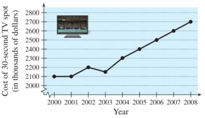
67. ADVERTISING The graph shows the average costs of a 30-second television spot (in thousands of dollars) during the Super Bowl from 2000 to 2008. (Source: Nielson Media and TNS Media Intelligence)

FIGURE FOR67

(a) Estimate the percent increase in the average cost of a 30-second spot from Super Bowl XXXIV in 2000 to Super Bowl XXXVIII in 2004.

(b) Estimate the percent increase in the average cost of a 30-second spot from Super Bowl XXXIV in 2000 to Super Bowl XLII in 2008.

68. ADVERTISING The graph shows the average costs of a 30-second television spot (in thousands of dollars) during the Academy Awards from 1995 to 2007.

(Source: Nielson Monitor-Plus)

(a) Estimate the percent increase in the average cost of a 30-second spot in 1996 to the cost in 2002. (b) Estimate the percent increase in the average cost of

a 30-second spot in 1996 to the cost in 2007.

69. MUSIC The graph shows the numbers of performers

who were elected to the Rock and Roll Hall of Fame from 1991 through 2008. Describe any trends in the data. From these trends, predict the number of performers elected in 2010. (Source: rockhall.com)

Year

Number elected

1991 1993 1995 1997 1999 2001 2003 2005 2007 2

4 6 8 10

1995 1997 1999 2001 2003 2005 2007

Year

Cost of 30-second

TV spot

(in thousands of dollars) 600

800 1000 1200 1400 1600 1800

200020012002 2003 2004 2005 2006 2007 2008

Year

Cost of 30-second

TV spot

(in thousands of dollars) 2000

2100 2200 2300 2400 2500 2600 2700 2800

1996 1998 2000 2002 2004 2006

Year

A

v

erage price

(in dollars per gallon) 2.60 2.80 3.00 3.20 3.40 3.60 3.80 4.00

5, 2

7, 6, 3, 6, 5, 8, ⫺7,⫺4

⫺2,⫺4,

⫺2, 2, ⫺7,⫺2,

x ( 3, 0)−

( 5, 3)−

( 3, 6)− ( 1, 3)−

3

units 6 units

3 1 5 7

y

x ( 1, 1)− −

( 2, 4)− − (2, 3)− 2 units

5

units

4

2

−2

−4

y

Year Sales (in millions)

2003 2007

(27)

70. LABOR FORCE Use the graph below, which shows

the minimum wage in the United States (in dollars) from 1950 to 2009. (Source: U.S. Department of Labor)

(a) Which decade shows the greatest increase in minimum wage?

(b) Approximate the percent increases in the minimum wage from 1990 to 1995 and from 1995 to 2009. (c) Use the percent increase from 1995 to 2009 to

predict the minimum wage in 2013.

(d) Do you believe that your prediction in part (c) is reasonable? Explain.

71. SALES The Coca-Cola Company had sales of $19,805 million in 1999 and $28,857 million in 2007. Use the Midpoint Formula to estimate the sales in 2003. Assume that the sales followed a linear pattern. (Source: The Coca-Cola Company)

72. DATA ANALYSIS: EXAM SCORES The table shows

the mathematics entrance test scores and the final examination scores in an algebra course for a sample of 10 students.

(a) Sketch a scatter plot of the data.

(b) Find the entrance test score of any student with a final exam score in the 80s.

(c) Does a higher entrance test score imply a higher final exam score? Explain.

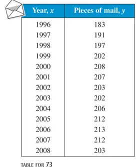
73. DATA ANALYSIS: MAIL The table shows the number

of pieces of mail handled (in billions) by the U.S. Postal Service for each year from 1996 through 2008.

(Source: U.S. Postal Service)

TABLE FOR73

(a) Sketch a scatter plot of the data.

(b) Approximate the year in which there was the greatest decrease in the number of pieces of mail handled. (c) Why do you think the number of pieces of mail

handled decreased?

74. DATA ANALYSIS: ATHLETICS The table shows the

numbers of men’s Mand women’s Wcollege basketball teams for each year from 1994 through 2007.

(Source: National Collegiate Athletic Association)

(a) Sketch scatter plots of these two sets of data on the same set of coordinate axes.

x

x y

y

x Year

Minimum wage (in dollars)

1950 1960 1970 1980 1990 2000 2010 1

2 3 4 5 6 7 8

Year,x Pieces of mail,y

1996 1997 1998 1999 2000 2001 2002 2003 2004 2005 2006 2007 2008

183 191 197 202 208 207 203 202 206 212 213 212 203

x 22 29 35 40 44 48 53 58 65 76

y 53 74 57 66 79 90 76 93 83 99

Year, x

Men’s teams,M

Women’s teams,W

1994 1995 1996 1997 1998 1999 2000 2001 2002 2003 2004 2005 2006 2007

858 868 866 865 895 926 932 937 936 967 981 983 984 982

(28)

(b) Find the year in which the numbers of men’s and women’s teams were nearly equal.

(c) Find the year in which the difference between the numbers of men’s and women’s teams was the great-est. What was this difference?

EXPLORATION

75. A line segment has as one endpoint and as its midpoint. Find the other endpoint of the line segment in terms of and

76. Use the result of Exercise 75 to find the coordinates of the endpoint of a line segment if the coordinates of the other endpoint and midpoint are, respectively,

(a) and (b)

77. Use the Midpoint Formula three times to find the three points that divide the line segment joining and

into four parts.

78. Use the result of Exercise 77 to find the points that divide the line segment joining the given points into four equal parts.

(a) (b)

79. MAKE A CONJECTURE Plot the points

and on a rectangular coordinate system. Then change the sign of the -coordinate of each point and plot the three new points on the same rectangular coordinate system. Make a conjecture about the location of a point when each of the following occurs.

(a) The sign of the -coordinate is changed. (b) The sign of the -coordinate is changed.

(c) The signs of both the - and -coordinates are changed.

80. COLLINEAR POINTS Three or more points are

collinearif they all lie on the same line. Use the steps below to determine if the set of points

and the set of points are collinear.

(a) For each set of points, use the Distance Formula to find the distances from to from to and from to What relationship exists among these distances for each set of points?

(b) Plot each set of points in the Cartesian plane. Do all the points of either set appear to lie on the same line?

(c) Compare your conclusions from part (a) with the conclusions you made from the graphs in part (b). Make a general statement about how to use the Distance Formula to determine collinearity.

TRUE OR FALSE? In Exercises 81 and 82, determine

whether the statement is true or false. Justify your answer.

81. In order to divide a line segment into 16 equal parts, you would have to use the Midpoint Formula 16 times.

82. The points and represent the

vertices of an isosceles triangle.

83. THINK ABOUT IT When plotting points on the

rectangular coordinate system, is it true that the scales on the - and -axes must be the same? Explain.

85. PROOF Prove that the diagonals of the parallelogram in the figure intersect at their midpoints.

x (0, 0)

( , )b c ( + , )a b c

( , 0)a

y y x

⫺5, 1 2, 11,

⫺8, 4,

C. A

C, B B, A

C2, 1 B5, 2,

A8, 3, C6, 3

B2, 6, A2, 3, y

x y

x

x 7,⫺3

⫺3, 5,

2, 1, ⫺2,⫺3,0, 0

1,⫺2,4,⫺1 x2,y2

x1,y1 ⫺5, 11,2, 4. 1,⫺2,4,⫺1

ym.

x1,y1,xm,

x2,y2 xm,ym

x1,y1

84. CAPSTONE Use the plot of the point in the figure. Match the transformation of the point with the correct plot. Explain your reasoning. [The plots are labeled (i), (ii), (iii), and (iv).]

(i) (ii)

(iii) (iv)

(a) (b)

(c)

x0, (d) ⫺x0,⫺y0

1 2y0

⫺2x0,y0 x0,⫺y0

x y

(x₀,y₀)

x y

(29)

Section 1.2 Graphs of Equations 13

The Graph of an Equation

In Section 1.1, you used a coordinate system to represent graphically the relationship between two quantities. There, the graphical picture consisted of a collection of points in a coordinate plane.

Frequently, a relationship between two quantities is expressed as an equation in two variables.For instance, is an equation in and An ordered pair is a solutionor solution pointof an equation in and if the equation is true when is substituted for and is substituted for For instance, is a solution of

because is a true statement.

In this section you will review some basic procedures for sketching the graph of an equation in two variables. The graph of an equationis the set of all points that are solutions of the equation.

Determining Solution Points

Determine whether (a) and (b) lie on the graph of

Solution

a. Write original equation.

Substitute 2 for xand 13 for y.

is a solution.

✓

The point doeslie on the graph of because it is a solution point of the equation.

b. Write original equation.

Substitute for xand for y.

is not a solution.

The point does notlie on the graph of because it is nota solution point of the equation.

Now try Exercise 7.

The basic technique used for sketching the graph of an equation is the

point-plotting method.

y⫽10x⫺7 ⫺1,⫺3

⫺1,⫺3 ⫺3⫽ ⫺17

⫺3 ⫺1

⫺3⫽? 10⫺1⫺7 y⫽10x⫺7

y⫽10x⫺7 2, 13

2, 13 13⫽13

13⫽? 102⫺7 y⫽10x⫺7

y⫽10x⫺7. ⫺1,⫺3

2, 13

Example 1

4⫽7⫺31 y⫽7⫺3x

1, 4 y.

b x a

y x a,b

y. x y⫽7⫺3x

1.2 G

RAPHS OF

E

QUATIONS

What you should learn

• Sketch graphs of equations. • Find - and -intercepts of graphs of

equations.

• Use symmetry to sketch graphs of equations.

• Find equations of and sketch graphs of circles.

• Use graphs of equations in solving real-life problems.

Why you should learn it

The graph of an equation can help you see relationships between real-life quantities. For example, in Exercise 87 on page 23, a graph can be used to estimate the life expectancies of children who are born in 2015.

y x

Sketching the Graph of an Equation by Point Plotting

1. If possible, rewrite the equation so that one of the variables is isolated on one side of the equation.

2. Make a table of values showing several solution points.

3. Plot these points on a rectangular coordinate system.

4. Connect the points with a smooth curve or line. When evaluating an expression

or an equation, remember to follow the Basic Rules of Algebra. To review these rules, see Appendix A.1.

(30)

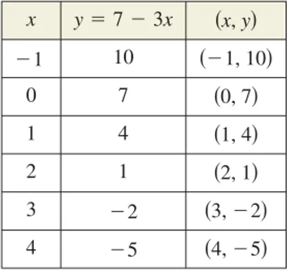
Sketching the Graph of an Equation Sketch the graph of

Solution

Because the equation is already solved for y, construct a table of values that consists of several solution points of the equation. For instance, when

which implies that is a solution point of the graph.

From the table, it follows that

and

are solution points of the equation. After plotting these points, you can see that they appear to lie on a line, as shown in Figure 1.14. The graph of the equation is the line that passes through the six plotted points.

FIGURE1.14

x (−1, 10)

(1, 4) (0, 7)

(2, 1)

(3,−2) (4,−5) y

−2

−4 ₋₂ 2 4 6 8 10

−4

−6 2 4 6 8

4,⫺5 3,⫺2,

2, 1, 1, 4, 0, 7, ⫺1, 10,

⫺1, 10 ⫽10

y⫽7⫺3⫺1

x⫽ ⫺1, y⫽7⫺3x.

Example 2

x y⫽7⫺3x x,y

⫺1 10 ⫺1, 10

0 7 0, 7

1 4 1, 4

2 1 2, 1

3 ⫺2 3,⫺2

(31)

Solution

Because the equation is already solved for begin by constructing a table of values.

Next, plot the points given in the table, as shown in Figure 1.15. Finally, connect the points with a smooth curve, as shown in Figure 1.16.

FIGURE1.15 FIGURE1.16

The point-plotting method demonstrated in Examples 2 and 3 is easy to use, but it has some shortcomings. With too few solution points, you can misrepresent the graph of an equation. For instance, if only the four points

and

in Figure 1.15 were plotted, any one of the three graphs in Figure 1.17 would be reasonable.

FIGURE1.17

x

−2 2

2 4

y

x

−2 2

2 4

y

x

−2 2

2 4

y

2, 2 1,⫺1,

⫺1,⫺1, ⫺2, 2,

x

2 4

−2

−4

2 4 6

(1,−1) (0,−2) (−1,−1)

(2, 2) (−2, 2)

(3, 7)

y=x2₋₂ y

x

2 4

−2

−4

2 4 6

(1,−1) (0,−2) (−1,−1)

(2, 2) (−2, 2)

(3, 7) y

y, y⫽x2_⫺_2.

Example 3

x ⫺2 ⫺1 0 1 2 3

y⫽x2_⫺₂ ₂ _⫺1 _⫺2 _⫺1 ₂ ₇

x,y ⫺2, 2 ⫺1,⫺1 0,⫺2 1,⫺1 2, 2 3, 7 One of your goals in this course

is to learn to classify the basic shape of a graph from its equation. For instance, you will learn that the linear equationin Example 2 has the form

and its graph is a line. Similarly, thequadratic equationin Example 3 has the form

(32)

Intercepts of a Graph

It is often easy to determine the solution points that have zero as either the -coordinate or the -coordinate. These points are called interceptsbecause they are the points at which the graph intersects or touches the - or -axis. It is possible for a graph to have no intercepts, one intercept, or several intercepts, as shown in Figure 1.18.

Note that an -intercept can be written as the ordered pair and a -intercept can be written as the ordered pair Some texts denote the -intercept as the -coordinate of the point [and the y-intercept as the -coordinate of the point ] rather than the point itself. Unless it is necessary to make a distinction, we will use the term interceptto mean either the point or the coordinate.

Finding x- and y-Intercepts Find the - and -intercepts of the graph of

Solution

Let Then

has solutions and -intercepts: Let Then

has one solution,

-intercept: See Figure 1.19. Now try Exercise 23.

0, 0 y

y⫽0. y⫽03_⫺₄₀ x⫽0.

0, 0,2, 0,⫺2, 0 x

x⫽±2. x⫽0

0⫽x3_⫺₄_x_⫽xx2_⫺₄ y⫽0.

y⫽x3_⫺₄_x_. y

x Example 4

0,b

y a, 0

x

x 0,y.

y

x, 0 x

y x y

x

y=x3−4x

x

4

−4

−2 4

(−2, 0) (0, 0) (2, 0) y

FIGURE1.19

x y

No -intercepts; one -interceptx y

x y

Three -intercepts; one -interceptx y

x y

One -intercept; two -interceptsx y

x y

No intercepts

FIGURE1.18

T E C H N O LO G Y

To graph an equation involving and on a graphing utility, use the following procedure.

1. Rewrite the equation so that is isolated on the left side.

2. Enter the equation into the graphing utility.

3. Determine a viewing windowthat shows all important features of the graph.

4. Graph the equation.

y y x

Finding Intercepts

1. To find -intercepts, let be zero and solve the equation for

2. To find -intercepts, let be zero and solve the equation for y x y. x. y

(33)

Symmetry

Graphs of equations can have symmetrywith respect to one of the coordinate axes or with respect to the origin. Symmetry with respect to the -axis means that if the Cartesian plane were folded along the -axis, the portion of the graph above the -axis would coincide with the portion below the -axis. Symmetry with respect to the -axis or the origin can be described in a similar manner, as shown in Figure 1.20.

x-axis symmetry y-axis symmetry Origin symmetry

FIGURE1.20

Knowing the symmetry of a graph beforeattempting to sketch it is helpful, because then you need only half as many solution points to sketch the graph. There are three basic types of symmetry, described as follows.

You can conclude that the graph of is symmetric with respect to the -axis because the point is also on the graph of (See the table below and Figure 1.21.)

y⫽x2_⫺_2. ⫺x,y

y

y⫽x2_⫺₂

(x,y)

(−x,−y)

x y

(x,y) (−x,y)

x y

(x,y)

(x,−y) x y

y x

x x

x

Graphical Tests for Symmetry

1. A graph is symmetric with respect to the x-axisif, whenever is on the graph, is also on the graph.

2. A graph is symmetric with respect to the y-axisif, whenever is on the graph, is also on the graph.

3. A graph is symmetric with respect to the originif, whenever is on the graph,⫺x,⫺yis also on the graph.

x,y ⫺x,y

x,y x,⫺y

x,y

Algebraic Tests for Symmetry

1. The graph of an equation is symmetric with respect to the -axis if replacing with yields an equivalent equation.

2. The graph of an equation is symmetric with respect to the -axis if replacing with yields an equivalent equation.

3. The graph of an equation is symmetric with respect to the origin if replacing with ⫺xand with y ⫺yyields an equivalent equation.

x ⫺x

x y

⫺y

y x

x ⫺3 ⫺2 ⫺1 1 2 3

y 7 2 ⫺1 ⫺1 2 7

x,y ⫺3, 7 ⫺2, 2 ⫺1,⫺1 1,⫺1 2, 2 3, 7 x

y=x2−2 y

(−3, 7) (3, 7)

(−2, 2) (2, 2)

(−1,−1) (1,−1) −4−3−2 2

−3 1

3 4 5 3

4 5 6 7

2

(34)

Testing for Symmetry

Test for symmetry with respect to both axes and the origin.

Solution

-axis: Write original equation.

Replace with Result is an equivalent equation.

-axis: Write original equation. Replace with

Simplify. Result is an equivalent equation.

Origin: Write original equation. Replace with and with

Simplify.

Equivalent equation

Of the three tests for symmetry, the only one that is satisfied is the test for origin symmetry (see Figure 1.22).

Using Symmetry as a Sketching Aid Use symmetry to sketch the graph of

Solution

Of the three tests for symmetry, the only one that is satisfied is the test for -axis sym-metry because is equivalent to . So, the graph is symmetric with respect to the -axis. Using symmetry, you only need to find the solution points above the -axis and then reflect them to obtain the graph, as shown in Figure 1.23.

Solution

This equation fails all three tests for symmetry and consequently its graph is not symmetric with respect to either axis or to the origin. The absolute value sign indicates that is always nonnegative. Create a table of values and plot the points, as shown in Figure 1.24. From the table, you can see that when So, the -intercept is

Similarly, when So, the -intercept is

1, 0. x

x⫽1. y⫽0

0, 1.

y y⫽1.

x⫽0 y

y⫽

x⫺1

.

Example 7 x

x

x⫺y2_⫽₁ x⫺⫺y2_⫽₁

x x⫺y2_⫽_1.

Example 6 y⫽2x3

⫺y⫽ ⫺2x3

⫺x. x ⫺y y ⫺y⫽2⫺x3

y⫽2x3

not y⫽ ⫺2x3

⫺x. x y⫽2⫺x3

y⫽2x3 y

not ⫺y.

y ⫺y⫽2x3

y⫽2x3 x

y⫽2x3 Example 5

x (1, 0)

(2, 1)

(5, 2)

x−y2= 1

2 3 4 5

2

1

−2

−1

y

FIGURE1.23

x y

2 2

1

−1

−2

−1

−2 y = 2x3

(−1,−2)

(1, 2)

FIGURE1.22

x

y = x− 1

2 3 4 5

−2

−3 −1

−2 2 3 5 4 6

y

(−2, 3)

(−1, 2) (3, 2)

(4, 3)

(0, 1) (2, 1)

(1, 0)

FIGURE1.24

x ⫺2 ⫺1 0 1 2 3 4

y⫽

x⫺1

3 2 1 0 1 2 3

x,y ⫺2, 3 ⫺1, 2 0, 1 1, 0 2, 1 3, 2 4, 3 In Example 7, is an

absolute value expression. You can review the techniques for evaluating an absolute value expression in Appendix A.1.