MTF DETERMINATION OF SENTINEL-4 DETECTOR ARRAYS
R. Reulkea∗, I. Sebastianb, C. Willigesb, R. Hohnb
aDepartment of Computer Science, Humboldt-Universitt zu Berlin, Germany - [email protected] b
Institut of Optical Sensor Systems, German Aerospace Center DLR, 12489 Berlin, Germany - (christian.williges, ilse.sebastian)@dlr.de b
Airbus Defense and Space, 85521 Ottobrunn, Germany - [email protected]
Commission I, WG I/10
KEY WORDS:PSF measurement, MTF evaluation, CCD, FPA, Sentinel-4
ABSTRACT:
The Institute for Optical Sensor Systems was involved in many international space projects in recent years. These include, for example, the fokal plane array (FPA) of the hyperspectral sensors ENMAP or Sentinel-4, but also the FPA for the high resolution FPA for Kompsat-3. An important requirement of the customer is the measurement of the detector MTF for different wavelengths. A measuring station under clean room conditions and evaluation algorithms was developed for these measurements. The measurement setup consist of a collimator with slit target in focus for illumination at infinity, a gimbal mounted detector facing an auxiliary lens in front, a halogen lamp with monochromator or filter, as well as optical and electrical ground support equipment. Different targets and therefore also different measurement and data evaluation opportunities are possible with this setup. Examples are slit, edge, pin hole but also a Siemens star. The article describes the measurement setup, the different measuring and evaluation procedures and exemplary results for Sentinel-4 detector.
1. INTRODUCTION
The Sentinel-4 payload is a multi-spectral camera system which is designed to monitor atmospheric conditions over Europe. The German Aerospace Center (DLR) in Berlin, Germany conducted the verification campaign of the Focal Plane Subsystem (FPS) on behalf of Airbus Defense and Space GmbH, Ottobrunn, Ger-many. In this publication, we will present in detail the MTF mea-surement set-up and data evaluation for deriving MTF at Nyquist frequency for the CCD 374 (UVVIS I and II) as well as CCD376 (NIR). A description of these back side illumination (BSI) detec-tors can be found in the publication (Jerram and Morris, 2016).
In this article, we focus on the MTF for the highest (ca.500nm) and lowest wavelengths (ca. 300nm) for the UVVIS detector. Because of subsurface diffusion effects we expect for BSI detec-tors the best results for the MTF at larger wavelengths.
The paper is organised as follows. First, a brief overview of the theory is given. The measurement setup is then described. In the next chapter the data evaluation and derivation of the MTF is described. Finally, a brief overview of the results is given. The paper comes up with conclusions and outlook.
2. PSF AND MTF
An overview of recent developments in scientific CCDs, in par-ticular front- and back-site illuminated CCDs, and the character-ization (including MTF measurements) of these devices can be found in (Lesser, 2015a) and (Lesser, 2015b). In (Swindells et al., 2014) an e2v imaging detector for the visible channel of the Euclid space telescope was described. This detector is an e2v back-illuminated, 4k x 4k, 12 micron square pixel CCD desig-nated CCD273-84. Results are presented also for MTF measure-ments, which shows a slight improvement with wavelength.
∗Corresponding author
An overview about PSF and MTF theory can be found in the book (Boreman, 2001) or (Jahn and Reulke, 2009). The PSF measure-ment is based on the definition of a translation invariant PSF:
V (x, y) =
The PSF can be calculated through the input signalU(x, y)and the measurement ofV(x, y). Conceptually, this is the shape of the blurred image of a point source (i.e., the blur spot). Together with PSF also Line Spread Function (LSF) and Edge Spread Function (ESF) can be derived:
• PSF from response of a point-like object (delta-function)
U x′, y′
=δ x′, y′
⇒ V(x, y) =H(x, y) (2)
• LSF from response of a line-like object (parallel to y-axis)
U x′, y′
In laboratory these three functions can be fully estimated with pinholes, tri-bars, slit or slanted edge (Reulke et al., 2011). As mentioned, Point Spread Function (PSF), Modulation Transfer Function (MTF) and Edge Spread Function (ESF) are mathe-matically related: The system MTF is the module of the Op-tical Transfer Function (OTF) derived as the 2D-Fourier Trans-form of the Point Spread Function and the derivative of the LSF with respect to position is Point Spread Function (PSF) in that direction. ESF or its normalized version of the Relative Edge Re-sponse (RER) and can be evaluated instead of the PSF or MTF. In real images the ESF from light to dark transitions was esti-mated using natural edges such as bridges or runways and it was assumed that the PSF had a normal distribution:
H(x) = 1
σH√2π ·e
−2σx2
H (5)
Thus, a first quantitative and shape description of the PSF is given by the parameterσH. Assuming for the PSF to a Gaussian distri-bution, the ESF is an error function:
y=p0
In this section, the measurement setup is to be investigated theo-retically more precisely.
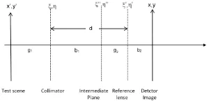
Figure 1. Measurement setup
Figure 1 shows the schematic sketch of setup. The test scene is imaged into the infinity by the collimator and focused on the detector by the reference lens. The collimator realise an image in the intermediate plane. From left to right we have the following amplitudes:
Amplitude in front of the collimator
UV
The amplitude in the intermediate plane is
UλZ(ξ′′,η′′)∼R Rdx′dy′H(1)
λ (ξ′′,η′′;x′,y′)·U E
λ(x′,y′) (8)
With the (amplitude) PSF of the collimator
Hλ(1)(ξ′′, η′′;x′, y′)∼ei·λπ·b1·(ξ
For incoherent radiation, we have
hUE
λ(x′,y′)·UλE∗(x′′,y′′)i=IλE(x′,y′)·δ(x′−x′′)·δ(y′−y′′) (10)
IE
λ (x′, y′)is the intensity of the incoherent Input radiation. In
the intermediate plane the intensity is
h(1)
The (intensity) PSF of the collimator. The amplitude in the image plane is
With the (amplitude) PSF of the test lens:
Hλ(2)(x, y;ξ′′, η′′)∼e
For incoherent radiation we have
IAλ(x,y)∼R Rdξ′′dη′′h(2)
For intensities we use the following equation
This is the (intensity) PSF of the entire system. It can not be represented as a convolution of two partial PSFs.
Therefore, we work with the following equation:
ˆ
Here the initial intensity is characterised by a hat for clarifying the incorrect calculation. From 20 one obtains the (incorrect) PSF of the optical overall system:
ˆ
The result of the calculation is, that large collimator aperture the result is independent from spatial frequency. Assuring that a suf-ficiently large aperture of the collimator is realised, the total MTF is determined only by the test lens. The collimator then has no effect on the MTF of the whole system.
3.2 Experimental Setup
The Optical Ground Support Equipment (OGSE) to be used for MTF measurement is located in a clean room class 100 000. The common set-up of CCD and the auxiliary lens optics Flektogon 2.8/20 facing the collimator has been illuminated by a slit at in-finity. The auxilary lens and the FPA are mounted together on a gimbal. Selected adjustment steps have to be performed to adjust the lens in a best focus position per wavelength in front of the CCD.
The collimator has a focal length of1200mmwith an aperture di-ameter of150mm. The lens optics has a focal length of20mm
and an aperture diameter of10mm. Due to the large ratio be-tween the two focal lengths, a displacement in front of the colli-mator in themmrange causes a displacement of the test object in front of the test object in theµmrange. The slit width and length in the image plane is8.7µm×130µm. Therefore we have ap-proximately 8 pixel in horizontal and about 5 pixel in vertical direction. With the short length of the slit, the derivation of the MTF is actually a 2D problem. However, one can start from the analysis of a 1D problem and evaluate the line spread function. In Figure 2 the signal in slit direction for a short slit is shown. In our case, we have aσ≈0.5. In this case the influence of the 2D problem is in the middle of the slit negligible and we can work with the 1D case.
Figure 2. Signal in slit direction for a short slit. The influence of the 2D problem is in the middle of the slit negligible
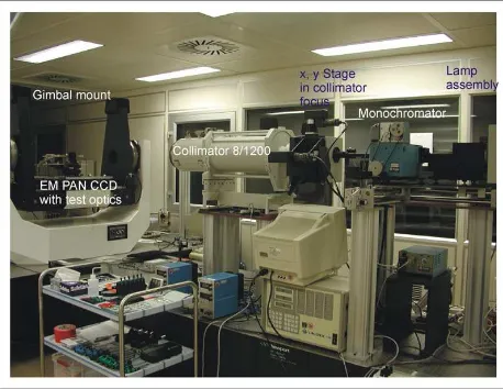
The slit target with geometric slit width of about1/10of a CCD pixel width will be located in collimator focus. The focus po-sition can be shifted by x- and y- step motors. The wavelength selection will be done by selecting a metal interference filter that is arranged between halogen lamp and collimator. Figure 3 illus-trates this set-up.
Figure 3. DLR Optical Ground Support Equipment
3.3 Lens Optics Flektogon 2.8/20 MTF measured by Schnei-der Kreuznach
Figure 4 shows the on-axis radial and tangential spectral MTFs of the Flektogon 2.8/20 measured by Schneider Kreuznach Optische Werke GmbH at 501 nm, 671 nm and 880 nm. For each spectral MTF measurement the individual best focus position has been adjusted in accordance with the dedicated procedure. The MTF curves will be used for MTF correction in a later step.
3.4 Detector
Figure 4. Spectral on-axis MTFs of the Flektogon 2.8/20 measured by Schneider Kreuznach
UVVIS Detector (see Figure 5)
Spectral range: 305nm−500nm
Pixel size (spatial):27.5µm
(spectral):15.0µm
With
- graded AR coating - thinned
- back side illuminated - no antiblooming capabilities
UVVIS I (Zone I)
Spectral range: 305nm−343nm
Split into:
UVVISIa: 305nm−316.5nm
UVVISIb: 316.5nm−343nm
With
- two outputs (used alternately) - different gains
- active pixels: 584pixels×255pixels
UVVIS II (Zone II)
Spectral range: 343nm−500nm
With - four outputs
- active pixels: 584pixels×1025pixels
3.5 Measurement Procedure
Figure 6 illustrates the principle of the measurement approach for the Sentinel-4 CCD. The slit image spot at infinity will be positioned perpendicular to CCD line or column direction. Sin-gle Pixel Illumination of a selected centre pixel is performed by measurement of signal at a certain pixel vs. slit step position.
The signal distribution for a certain pixel position is shown in Figure 7. The slit length is about 8 pixel in vertical direction and 5 pixel horizontal direction. At each pixel position at least 10 measurements are available, which are related to a known slit position.
In order to analyse signal stability, the signal was measured ap-proximately 30 times for each slit position (see Figure 8). The figure shows that the time dependency has no visible drift. Mean
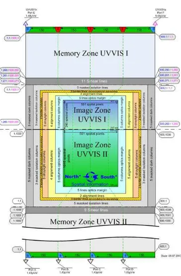
Figure 5. UVVISII detector
Figure 6. Measurement Procedure
and standard deviation for each measured value at different pixel positions is shown in Figure 9.
In Figure 9 the signal distribution, measured on different single pixel, is evaluated later for MTF determination. The error bars were also plotted. It can be seen clearly that the standard devia-tion of the measured signals is very small.
In the Figure 10 the variation of the signal from 77 measurements (slit steps) was analysed for different pixel around a predefined centre pixel in spatial and spectral direction. The PRNU of the detector, but in particular the spatial variation of the illumination, is responsible for the large change in the amplitude.
3.6 Data Evaluation
Figure 7. Signal distribution over the UVVISI detector with slit in vertical direction
Figure 8. Signal over time for different slit positions
Figure 9. Signal at different slit positions
Figure 11 shows the signal in dependence of pixel position. We have also analysed the 1-sigma uncertainty of the signal. From the illustration it becomes clear that the drift and noise is negligi-ble.
For the further data evaluation the zero point correction is nec-essary (see green line in Figure 11). The waveform close to the maximum of the signal differs significantly between the two spec-tral channels. The distinct structure in the long-wave specspec-tral range has effects on the frequency response of the MTF above
Figure 10. Spectral PSF: In horizontal or spatial direction (upper image) and in vertical or spectral direction (lower image).
Figure 11. Signal distribution over a pixel (305nmleft,495nm
right). Green line is a zero-point correction
the first zero of the sinc function.
4. RESULTS
The evaluation was carried out in a region of3×3pixels around the centre pixel. In figure 12 the MTF from this 9 pixel are plot-ted. The thick green line is the expected MTF shape, derived from the optics-, slit- and pixel MTF. It is clear from Frigure 12 that the influences of pixel size, optics and slit size are sufficient for describing the measurement signal. The 9 measurements also show that the MTF variation is in a few percent range.
In Figure 13 the correction by optics and slit MTF of the MTF is visible in the spatial and spectral directions. The results are close to the physical limit of the pixels MTF (63%). In addition, error bars were plotted in order to characterise the standard deviation of the individual measuring points.
The results are summarised below. For this purpose, the MTF was analysed as a function of the signal (see Table 1) and the wavelength (Table 2). (In the table, earlier studies were also in-cluded.)
Figure 12. Uncorrected MTF (at305nm) in comparison to theoretical influences. Spectral diection (upper image,15µm)
and spatial direction (lower image27.5µm).
Figure 13. MTF (at305nm) in spectral (upper image,15µm) and spatial direction (lower image27.5µm)
5. CONCLUSION AND OUTLOOK
In the paper, a generic approach for the determination of MTF of detectors with a slit function was presented. The operability of the approach was shown by means of some examples. It has been shown that the derived MTF is within the expected range.
Signal MTF (mean) MTF (Std.dev)
8TDN 61.9% 0.7%
14TDN 61.3% 0.6%
60TDN 60.9% 0.6%
Table 1. Signal dependence (spatial direction,495nm) at Nyquist Frequency
Wave- Spectral Spatial
lenght (mean) (std.dev.) (mean) (std.dev.)
305nm 59.2% 1.9% 56.6% 1.1%
340nm 58.4% 56.1%
400nm 59.2% 55.7%
495nm 60.9% 0.7% 58.2% (VIS2)
Table 2. Spectral and spatial MTF dependence at Nyquist Frequency
Although most of the results of an MTF derivation @Nyquist are around60%, we had no single result above the63%limit. This could be an indication of the correctness of the evaluation. There were also no abnormalities in intensity and spectral dependence.
The resulting detector MTF shall fulfils the following require-ment over the full spectral range of the UVVIS CCD:
• In the27.5µmdirection the (spatial) MTF shall be better 58%@Nyquist.
• In the15.0µmdirection the (spectral) shall be better45% @Nyquist.
The MTF in the spatial direction almost meets the requirements. (The real results are between56%and58%). However, the MTF in the spectral direction is clearly better than required. (Between 58%and61%.)
Open issues are related with
• the analysis of asymmetries and conspicuously structure on measured signal form and the influence on the MTF and,
• the effect that the MTF in the spatial direction is2%−3% smaller than in the spectral direction.
ACKNOWLEDGEMENTS
The presented work has been performed under ESA contract. The authors would like to express their thanks to their respective col-leagues at Airbus Defense and Space, ESA and EUMETSAT, and to all partner companies within the SENTINEL 4 industrial con-sortium for their valuable contributions to the continuing success of this very challenging program. This article has been produced with financial assistance of the EU. The views expressed herein shall not be taken to reflect the official opinion of the EU.
REFERENCES
Boreman, G. D., 2001. Modulation transfer function in optical and electro-optical systems. Vol. 21, SPIE press Bellingham, WA.
Jahn, H. and Reulke, R., 2009. Systemtheoretische Grundlagen optoelektronischer Sensoren. John Wiley Sons.
Jerram, P. and Morris, D., 2016. Recent sensor designs for earth observation. Vol. 9881, pp. 988111–988111–14.
Lesser, M., 2015a. A summary of charge-coupled devices for as-tronomy. Publications of the Astronomical Society of the Pacific
127(957), pp. 1097.
Lesser, M., 2015b. A summary of charge-coupled devices for as-tronomy. Publications of the Astronomical Society of the Pacific
127(957), pp. 1097.
Reulke, R., Brunn, A. and Weichelt, H., 2011. Spatial resolution assessment from real image data.