Phase-space analysis of daily streamflow:
characterization and prediction
Q. Liu
a, S. Islam
a ,*, I. Rodriguez-Iturbe
b& Y. Le
a aThe Cincinnati Earth System Science Program, Department of Civil and Environmental Engineering, University of Cincinnati, PO Box 210071, Cincinnati, OH 45221-0071, USA
b
Department of Civil Engineering, Texas A&M University, College Station TX 77843, USA
(Received 7 May 1996; revised 17 January 1997; accepted 3 February 1997)
This paper describes a methodology, based on dynamical systems theory, to model and predict streamflow at the daily scale. The model is constructed by developing a multidimensional phase-space map from observed streamflow signals. Predictions are made by examining trajectories on the reconstructed phase space. Prediction accuracy is used as a diagnostic tool to characterize the nature, which ranges from low-order deterministic to stochastic, of streamflow signals. To demonstrate the utility of this diagnostic tool, the proposed method is first applied to a time series with known characteristics. The paper shows that the proposed phase-space model can be used to make a tentative distinction between a noisy signal and a deterministic chaotic signal. The proposed phase-space model is then applied to daily streamflow records for 28 selected stations from the Continental United States covering basin areas between 31 and 35 079 km2. Based on the analyses of these 28 streamflow time series and 13 artificially generated signals with known characteristics, no direct relationship between the nature of underlying streamflow characteristics and basin area has been found. In addition, there does not appear to be any physical threshold (in terms of basin area, average flow rate and yield) that controls the change in streamflow dynamics at the daily scale. These results suggest that the daily streamflow signals span a wide dynamical range between deterministic chaos and periodic signal contaminated with additive noise. q 1998 Elsevier Science Limited. All rights
reserved
1 INTRODUCTION
The classical approaches for analyzing hydrologic signals (i.e. streamflow, rainfall, etc.), whether they are produced by a deterministic or stochastic process, are based on: (i) exploring the observable to detect patterns; (ii) constructing an explanatory model from first principles; and (iii) measur-ing data to initialize, calibrate and validate the model. In characterizing streamflow, one could argue that basic equations (e.g. for rainfall-runoff transformations, overland flow, hydraulic routing) are well known and can be derived for idealized conditions. However, these idealized condi-tions are far from being physically realistic, especially from the viewpoint of space–time heterogeneity. Even if we accept that model equations can be formulated for idealized conditions, correct specification of initial and
boundary conditions would require measurements of state variables in a four-dimensional volume. However, measure-ments are usually taken only at discrete locations and times. The inherent spatial and temporal variability in streamflow make the basic equations only an approximation whose values in operational hydrology is conditional on appropri-ate calibration through numerous tuning parameters.
An alternative approach is to construct a streamflow model directly from the available data. A key assumption behind constructing such a model is that even if the exact mathematical description of a dynamical system is not known, the state space can be reconstructed from a single variable time series1. The state space is defined as the multi-dimensional space whose axes consists of variables of a dynamical system. For example, for a three-variable model, the state space will be three dimensional and each of the three axes will be represented by a model variable. When the state space is reconstructed from a time series,
Advances in Water Resources21(1998) 463–475
q1998 Elsevier Science Limited All rights reserved. Printed in Great Britain 0309-1708/98/$19.00 + 0.00
PII: S 0 3 0 9 - 1 7 0 8 ( 9 7 ) 0 0 0 1 3 - 4
463
rather than with actual model variables, it is customary to call this state space a phase space. We will use a time-delay embedding (defined in Section 2) to reconstruct the phase-space from the observed streamflow signals. In principle, the phase space contains the knowledge about the internal dynamics of the system and thus can be used as a predictive tool. The basic idea here is that since the embedding map preserves the underlying dynamic structure, the future can be predicted from the behavior of the past. As shown by Takens2, the phase space retains essential properties of the original state space including the dimensionality of the underlying system. Now, if one can reconstruct the determi-nistic rules underlying the data in a phase space then one can attempt to predict the future states from the history of the data embedded in the phase space. Several recent studies have successfully used phase-space-based models for chaotic signal characterization3–5, prediction6, noise reduc-tion7and lake level prediction8. In addition, as we will see, a phase-space-based model can also be used to make short-term prediction and provide a tentative distinction between low-dimensional determinism and noise9,10.
Hydrologists have long maintained that large basins are smoother in their streamflow response behavior than small basins. This assumption has not been really substantiated from a quantitative, data based, point of view, although arguments based on the smoothing effect resulting from larger storage property constitute a reasonable basis for its acceptance. Such a smoothing effect of large basins is fre-quently translated in the assertion that because of their inherent larger degree of linearity, their response (e.g. run-off) is easier (compared to the smaller basins) to predict. It is commonly argued that as the time and spatial averaging increase, then the rainfall–streamflow relationships may become more linear and hence the streamflow becomes more predictable. However, even if the above is true, it is not clear how much the predictability of streamflow will increase in terms of accuracy and prediction lead time. Recent studies have shown possible presence of chaos in streamflow11,12. If the underlying streamflow signal is chaotic, it is quite possible that its inherent predictability will be quite limited irrespective of the basin area.
In this study, we will describe an alternative model for streamflow prediction. This model will be used to investi-gate the characteristic signatures of streamflow signals (e.g. low-order determinism vs stochastic noise) at the daily scale. For example, does streamflow change dynamics (non-linear to (non-linear) with increasing basin area? What is the impli-cation of the nature of streamflow characteristics on its predictability? We will use recent developments in nonlinear modeling, phase-space reconstruction from a time series and related diagnostic tools to address the above issues.
2 STREAMFLOW MODELING: A DYNAMICAL SYSTEM PERSPECTIVE
Due to the dramatic expansion of digital data acquisition
and processing, it is now possible to develop predictive models for streamflow dynamics from a ‘theory-poor’ and ‘data-rich’ perspective. By theory-poor we mean that our approach does not require explicit formulation of governing partial differential equations. The idea of data intensive modeling is by no means new—an autoregressive model13,14is a good example. What is new is the emergence of a set of concepts and tools (such as phase-space recon-struction, neural network, etc.) that combine broad approxi-mation abilities and few specific assumptions15. We will take this data-rich and theory-poor perspective to construct a predictive model directly from streamflow time series. Building this type of dynamical model from a time series involves two steps: (i) reconstruction of the phase space from data by time delay embedding; and (ii) development of a methodology for phase-space prediction.
2.1 Reconstruction of the phase space from data by time delay embedding
LetX0(t) be the time series of a dynamical variable from a
potentially complex natural system (e.g. streamflow signal). As theM variables {Xk(t)} describing the system satisfy a
set of first-order differential equations, successive differen-tiation in time reduces the problem to a single highly non-linear differential equation of Mth order for one of these variables. Thus, instead of Xk(t), k ¼ 0, 1,…M ¹ 1, we
may useX0(t), the variable of the time series data, and its
(M¹1) successive derivativesX(0k)(t),k¼1,…M¹1, to be theMvariables of the problem spanning the phase space of the system1. Therefore, in principle, sufficient information is given in a one-dimensional time series to construct a multidimensional phase-space for studying the system dynamics.
A simple procedure, suggested originally by Ruelle16, avoids the problem of calculating X0(k)(t) from a time series ofX0(t) and uses multiple time delays as a surrogate
for successive derivatives. A point in an M-dimensional phase-spaceX0(t) is then defined as
X0(t)¼[X0(t), X0(tþt), X0(tþ2t), …,
3X0{tþ(M¹1)t}]
To construct a well-behaved phase space by time delay, a careful choice of t is critical. A popular choice for this
characteristic time scale is chosen from the autocorrelation function of the original time series. Here, the time delaytis
[Fig. 1(b)]. A phase-space plot of the Henon map and a white noise sequence in Fig. 2, on the other hand, reveals remarkable structure in the chaotic Henon map while the white noise sequence fills up the entire plane with no apparent structure.
2.2 Develop a methodology for phase-space prediction
Once we have reconstructed the phase space, we can use some of its properties to develop a short-term prediction model. For example, if the underlying dynamics is determi-nistic, then the order with which the points in the phase space appear will also be deterministic. Thus, we may be able to define some functional relationship between the current stateX(t) and the future statesX(tþP), i.e. X(tþ P) ¼ Fp(X(t)). Now, we need to find a predictor Fp that
approximates Fp. There are a variety of numerical
tech-niques to approximate Fp from scattered points in the
phase space. This methodology can be illustrated by using
Fig. 3, where part of a trajectory is shown in a two-dimensional phase-space and the present state is denoted by an open circle. The solid circles indicate neighbors of the current state, and the arrowheads show movement of the neighbors through a local section of the phase space. By finding a suitable function (linear or nonlinear) that approxi-mates how the neighbors move, a prediction of the current state can be made. This is know as local approximation as opposed to a global approximation which defines a functional relationship over the entire phase space.
Farmer and Sidorowich6introduced local linear models for phase-space forecasting. Smith2discussed the relation-ship between local linear and nonlinear models as well as between the local and global approaches. In general, local linear approximation has been shown to provide better prediction accuracy for a number of controlled datasets18. In this paper, local approximation methods will be used. One such method, popularly known as the nearest neighbor method, approximates unknown functions near the present
Fig. 1.(a) Time series of 100 points for the chaotic Henon map:xtþ1¼1¹ax2tþyt;ytþ1¼bxtwitha¼1.4 andb¼0.30. This time series
is in many ways indistinguishable from random noise. (b) Time series of 100 points generated from uniform distribution in the interval between 0 and 1.
state vector by using the nearest neighbor of the present state.
We now locate nearbyM-dimensional points in the phase space and choose a minimal neighborhood withK closest neighbors such that the predictee (the point from which the prediction is made) is contained within the smallest simplex. To enclose a point in anM-dimensional space, we require a simplex with a minimum ofMþ1 points. Then, to obtain a prediction, we project the domain of the chosen nearest neighborsTP (prediction step) steps forward and compute
Fpto get the predicted value. Since it becomes increasingly
difficult to define an enclosing simplex for higher dimen-sional embedding spaces, we have extended the above idea to the nearest neighbors in an Euclidean sense. A minimum of M þ 1 nearest neighbors are chosen based on the Euclidean distance between the neighbor and the predictee. Then, we project the domain of the chosen neighborsTpstep
forward and estimate the predicted value. We have explored several estimation kernels including arithmetic average, weighted average and weighted regression to estimate the predicted value. It was found that arithmetic average provides comparable prediction accuracy and requires no tuning parameters and hence we have chosen arithmetic average of projected neighboring points to obtain the predicted value in this study.
There are only two parameters to be chosen for this phase-space prediction model: embedding dimension M, and number of nearest neighbors K. In general, Mmin .
(2Dþ1) whereDis the attractor dimension. An estimate of the attractor dimension may be obtained from the corre-lation dimension4,5. Prediction results are sensitive to the choice of M10. We will look at the prediction accuracy (correlation between predicted and observed) as a function of embedding dimension to choose an optimum value ofM
for our prediction algorithm. Since to enclose a point in an
M-dimensional space, we require to construct a simplex with a minimum of (Mþ1) points, one hasKmin.(Mþ1).
Use of the phase space to develop a forecasting model may appear to be similar to an autoregressive model: a pre-diction is estimated based on time-lagged vectors. However, the crucial difference is that understanding phase-space geometry frames forecasting as recognizing and then repre-senting underlying dynamical structures. For example, two
neighboring points in a phase space may not be close to each other within the context of a time sequence. The traditional autoregressive (AR) model relies on time-lagged signals that are neighbors in a temporal sense, whereas a neighbor in a phase space is close in a dynamic sense. In addition, once the number of lags exceeds the minimum embedding dimension, the geometry of the underlying dynamics will not change. A global linear model, such as the AR model, must do this with a single hyperplane with no fundamental insight into the underlying geometric structure. Unlike traditional AR models, the proposed methodology also promises to make a tentative distinction between stochastic noise and low-dimensional chaos. A characteristic feature of chaotic dynamics is that the prediction accuracy exponen-tially decays as the prediction time increases. On the other hand, for a noisy system the prediction accuracy does not decay sharply with prediction lead time9,10.
2.3 Distinction between deterministic chaos and stochastic noise
Below, we show how a phase-space-based forecasting model works by applying it to a known chaotic time series generated from the well-studied chaotic Henon map. Additionally, as an example of noisy dynamics, we study uncorrelated additive noise superimposed on a sine wave. Such uncorrelated noise can be thought of as measurement error superimposed on a hypothetical streamflow signal with a pronounced seasonal cycle. We have used a total of 5000 points for each time series; the first 4000 points are used as a training set while the other 1000 points are used to make predictions and estimate prediction accuracy as a function of prediction lead time.
Fig. 4 shows the prediction accuracy for the chosen
Fig. 3.Schematic representation of the nearest-neighbor method for phase-space-based prediction. The present state X(t) and its unknown future valueX(tþT) are denoted by open circles, while the black dots inside the circle represent the neighborhood ofX(t) in the phase space. By finding a suitable function (linear or non-linear) that approximates how neighbors move, a prediction of the
current state is made6,19.
Fig. 4.Prediction accuracy, defined as the correlation between the observed and predicted values of a particular time series, as a function of prediction lead time. The dotted line represents a sinewave with additive noise, while the solid line depicts the
chaotic and noisy time series. Here, the prediction accuracy is defined as the correlation between the observed and pre-dicted values of a particular time series. The dotted line shows that the correlation does not decline for additive noise (here white noise is superimposed on a periodic signal) as one tries to forecast further into the future. In contrast, the solid line (for a time series generated from a chaotic Henon map) shows the declining signature charac-teristic of a chaotic sequence. For a detailed discussion on the Henon map including its stability and phase-space characteristics we refer to Ref.19. The correlation coeffi-cient of the Henon map prediction drops abruptly from 0.95 for Tp¼ 1 to 0.16 forTp¼ 3. Such a sharp drop in the
prediction accuracy is a characteristic signature of a chaotic signal. If there is a periodicity in the signal which is less than the maximum prediction lead time then the effects of the periodicity of the signal will show up in the prediction accuracy. To avoid such an influence, usually a difference time series is used9,10. On the other hand, the correlation coefficient for the noisy time series does not show such an exponential loss of information with prediction lead time. In
the following section, we will explore the utility of this diagnostic tool to characterize the nature of daily streamflow.
3 PHASE-SPACE-BASED MODEL FOR STREAMFLOW PREDICTION
3.1 Analysis of daily streamflow from the southwestern United States
The dataset used in this study is described by Walliset al.20. It consists of daily streamflow measurements from 1948 to 1988 for 1009 streamgages across the United States. All files are serially complete for 41 water years beginning in October 1948 and ending in September 1988. Missing data in the raw data records are estimated using simple prorating methods described in Walliset al.20.
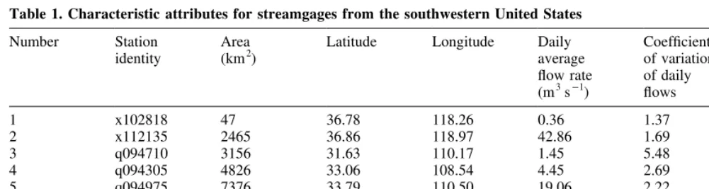
First, eight stations are chosen from the southwestern United States covering three states: Arizona, California and New Mexico. Relevant information for eight selected
Table 1. Characteristic attributes for streamgages from the southwestern United States
Number Station
identity
Area
(km2) Latitude Longitude Dailyaverage flow rate (m3s¹1
)
Coefficient of variation of daily flows
Average yield (105m day¹1)
1 x102818 47 36.78 118.26 0.36 1.37 66.10
2 x112135 2465 36.86 118.97 42.86 1.69 150.20
3 q094710 3156 31.63 110.17 1.45 5.48 3.97
4 q094305 4826 33.06 108.54 4.45 2.69 7.97
5 q094975 7376 33.79 110.50 19.06 2.22 22.32
6 x094420 10381 32.97 109.31 5.21 2.97 4.33
7 q094985 11148 33.62 110.92 24.52 2.61 19.00
8 q094485 20442 32.87 109.51 13.16 3.51 5.56
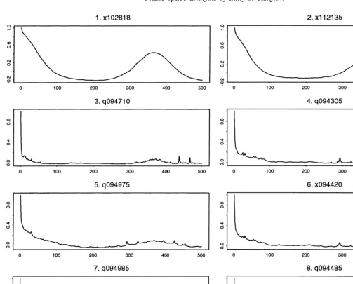
Fig. 5.Daily time series of eight streamflow records from the southwestern United States described in Table 1, for 41 years (1948–1988). The vertical axis is flowrate (m3s¹1
stations used in this study is summarized in Table 1. Here, basin yield is defined as the average flow rate per unit area. These stations are chosen to represent a wide range of basin areas from the same geographical region. Basin areas for the selected stations range between 47 and 20 442 km2. Station IDs with letter prefix ‘q’ indicates that there were no data gaps for the station in the raw USGS data file, while a prefix ‘x’ indicates that there were periods of missing data that were estimated by Walliset al.20.
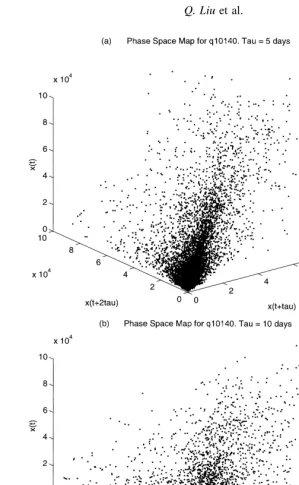
Fig. 5 shows the variations of daily streamflow values for the eight streamflows for 41 years. It appears that the smaller basins (1 and 2) seem to have a pronounced annual cycle while the larger basins (3–8) do not show appreciable annual cycle. This feature can be clearly seen in Fig. 6, which shows the streamflows for the smallest and the largest basins during the first 5 years (1948–1953). The autocorrelation function for the selected eight basins are shown in Fig. 7. It appears that the two smallest basins (1 and 2) show apparent periodicity, while the other six do not show any clear periodic signature. This preliminary analysis suggests that streamflow records 1 and 2 are dominated by a seasonal cycle with added noise. On the other hand, a sharp decay in the autocorrelation function for the other six streamflow records suggests that their dynamics might be controlled either by random processes or by deterministic chaos. We will use phase-space model-based predictions to make a distinction between these two types of streamflow characteristics. Fig. 8(a) and (b) show three-dimensional phase-space maps for q10140 with two different values of lag time (t). If the dimension of the underlying attractor is
greater than three, a phase-space map in a three or lower dimension would appear as a cluster of points with no identifiable structure. It appears that the underlying dynamics for this time series (q10140) has a higher
dimensional attractor, and consequently the underlying structure is hidden. However, a higher dimensional phase-space map, although difficult to visualize, is expected to show structured pattern in the phase space.
As discussed in Section 2, the first step in developing a phase-space model for streamflow signals involves the determination of optimum embedding dimensions from the daily streamflow time series. This is done by plotting the correlation coefficient between the observed and pre-dicted streamflows forTp¼1 (1-day ahead prediction) as
a function of embedding dimension. Fig. 9 shows the correlation coefficient for eight streamflows as a function of embedding dimension, M. We choose the optimum embedding dimension such that it produces the largest correlation coefficient for 1-day ahead prediction. For example, streamflow record 5 produces a maximum corre-lation coefficient of 0.85 for M ¼ 4 and hence for this
streamflow four is chosen as the optimum embedding dimension. Optimum embedding dimensions found were 2, 3, 3, 4, 4, 7, 2 and 4 for streamflow records 1–8, respec-tively. An estimate of optimum embedding dimension provides an indication of the underlying complexity of the system. For example, in general, the larger the embedding dimension the greater is the underlying complexity. There is no apparent trend between the optimal embedding dimension and basin area. With these embedding dimension estimates, we are now set to make predictions.
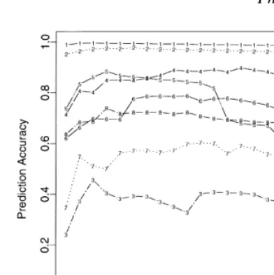
Fig. 10 shows the prediction accuracy for the selected stations as a function of the prediction lead time. For each of these streamflows we have made 1-day to 20-day ahead predictions. The two smallest basins show a very high degree of correlation between the observed and the pre-dicted sequence. This persistence in prediction accuracy may be considered analogous to periodic signal with
additive noise, as seen in the illustrative example of Fig. 4. Prediction accuracy for the other six stations show an exponential decay with the prediction lead time. Sugihara
et al.10argued that such an exponential decline in prediction accuracy could arise from locally exponentially diverging trajectories and could be taken as an operational definition of chaos. A sharp decay of correlation between the observed and predicted streamflow records shown in Fig. 10 could thus suggest a possible presence of deterministic chaos. This serves as a preliminary evidence that the daily streamflow time series analyzed here show a change in dynamics as we increase the basin area. It appears to show a tendency to go from noisy dynamics to chaotic dynamics for increasing basin areas. As we explain below, the influence of other factors such as climate, topography, vegetation and soil texture could complicate this apparent relationship between basin area and streamflow characteristics.
A direct implication of the results reported above is that increasing basin area does not necessarily imply increased linearity or enhanced predictability. This is somewhat counterintuitive. One could argue that a larger basin
would spatially average small-scale fluctuations in forcing functions (e.g. rainfall) and basin attributes (e.g. spatial variability in topography, soil texture). This averaging should reduce the dimension of the underlying dynamical system and consequently lead to increased streamflow pre-dictability. There does not appear to be any consistent reduction in the optimum embedding dimension as we increase the basin area. Another feature to note for these eight stations is that there appears to be a relationship between the yield (average flow rate per unit area expressed as depth per day) and basin dynamics. For higher yield, basin dynamics appear to be more predictable, whereas for lower yield it becomes more unpredictable. If one looks at the geographical locations of these basins, basins 1 and 2 are seen in the Sierra Nevada while the other six basins appear to be in the Gila and Salt River drainages. The Sierra Nevada area is dominated by winter storm fronts coming from the Pacific, and snow accumulation and snowmelt play a strong role in the hydrology of streamflow records 1 and 2. The streamflow records 3–8, on the other hand, are affected by more variable winter storms,
by small-scale convective events, and by occasional intense, large area summer monsoons. Hence, there tends to be less persistence in these streamflow signals. Based on these hydrometeorological explanations, one could argue that shift in streamflow characteristics from noisy dynamics to low-dimensional determinism are sig-nificantly affected by variability and timing of atmo-spheric processes in this region. This, however, complicates the notion of increased linearity or enhanced predictability of streamflow with increasing area. As the results and inferences presented above are based on the analysis of eight select stations from a geographical region, further analysis with more streamgages from other regions are required before a generalized conclusion can be attempted.
3.2 Analysis of daily streamflow from the continental United States
In this section, we analyze daily streamflow data from 20 streamgages from across the continental United States. These streamgages are chosen from the data set compiled by Wallis et al.20. Relevant information for 20 select stations used in this study are summarized in Table 2. These stations were chosen randomly to represent a wide range of basin areas from different geographical regions within the continental United States. Basin areas for the selected stations range between 31 and 35 079 km2. This is the widest range, in terms of basin area, we could find for unregulated streams. For these stations average flow rate varies over three order of magnitudes with a range between
0.30 and 343 m3s¹1
. The yield varies between 1.64 and 244.8 3 10¹5
m day¹1
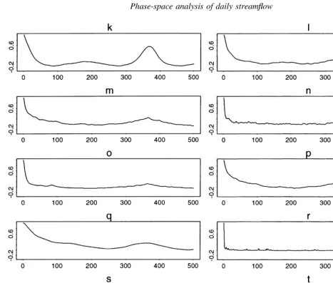
. For the streamflow time series analyzed, there does not appear to be any relationship between the basin area and the coefficient of variation or the basin area and the yield. Fig. 11 shows the autocorrelation coefficient for these 20 streamflow time series. There does not appear to be any direct relationship between apparent periodicity in the autocorrelation function and the basin area.
Now we will use phase-space model based predictions to explore whether there is a physical threshold, in terms of basin area, at which the dynamics of streamflow change from linear noisy dynamics to chaotic dynamics for
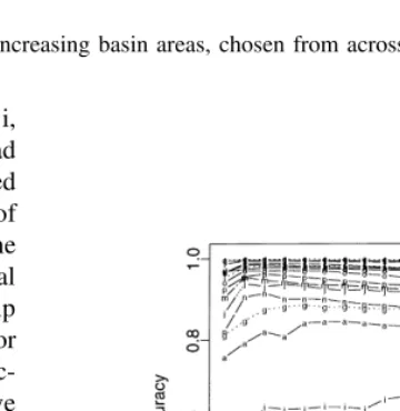
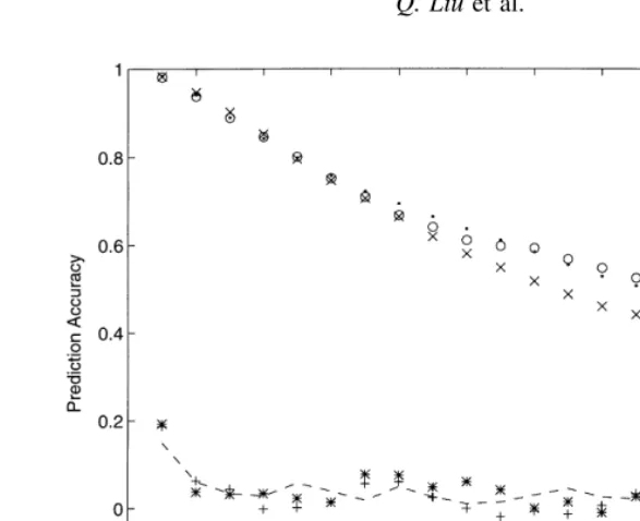
increasing basin areas. Fig. 12 shows the prediction accuracy for 20 streamflows as a function of embedding dimension. As before, we use this figure to choose the opti-mum embedding dimension such that it produces the largest correlation coefficient for 1-day ahead prediction. Fig. 13 shows the prediction accuracy for these 20 stations as a function of the prediction lead time. For each of these streamflows we have made 1-day to 20-day ahead predictions.
Four basins (d, f, q and t) show persistent high correlation between the observed and the predicted sequence. This persistence in prediction accuracy is analogous to periodic signal with additive noise, as seen in the illustrative example
Fig. 9.Prediction accuracy as a function of embedding dimension for the selected eight streamgages from the southwestern United
States.
Fig. 10.Prediction accuracy as a function of prediction lead time for 1-day to 20-day ahead predictions for the eight streamgages
from the southwestern United States.
Table 2. Characteristic attributes for streamgages selected from the continental United States
Number Station
a q10730 31 43.15 ¹70.97 0.56 1.55 156.07
b q20990 39 36.04 ¹79.95 0.50 3.24 110.76
c q54540 65 41.69 ¹91.49 0.45 3.52 93.25
d x133295 78 45.34 ¹117.29 2.21 1.25 244.80
e q73730 132 31.54 ¹92.41 1.72 3.65 112.58
f x22670 153 27.96 ¹81.50 1.33 0.61 75.11
g q53935 212 45.45 ¹89.98 2.36 2.06 96.18
h q69115 287 38.61 ¹95.64 1.58 5.70 47.56
i q54660 401 41.27 ¹90.38 2.91 2.54 62.69
j q54640 13322 42.50 ¹92.33 77.02 1.57 4.99
k q10140 14666 47.26 ¹68.59 268.32 1.44 158.07
l q53405 16155 45.41 ¹92.65 132.85 1.09 6.76
m q54645 16854 41.97 ¹91.67 99.82 1.38 51.17
n x69020 17812 39.64 ¹93.27 101.88 2.34 49.42
o q54650 20154 41.41 ¹91.29 124.67 1.23 53.45
p q23205 20400 29.96 ¹82.93 213.58 0.83 90.45
q q64855 21809 42.83 ¹96.56 25.94 2.84 10.27
r q80805 22772 33.01 ¹100.18 4.32 7.16 1.64
s q21310 22860 34.20 ¹79.55 288 0.84 108.8
of Fig. 4. Prediction accuracy for seven stations (b, c, e, h, i, n and r) shows an exponential decay with the prediction lead time. This sharp decay of correlation between the observed and predicted streamflows suggests the existence of deterministic chaos. Prediction accuracy for the other nine stations falls somewhere between these two dynamical regimes. There does not appear to be any direct relationship between the area or yield and the prediction accuracy. For example, the largest basin (t) shows persistence in predic-tion accuracy similar to a periodic signal with additive noise, while the third largest basin (r) shows a dynamical behavior similar to a deterministic chaos and the second largest basin (s) falls somewhere in the middle.
To explore the origin of such mixed characteristics, low-order determinism to stochastic noise, for different stream-flows, we now focus on a series of synthetically generated time series with known dynamics. We have generated 13 time series with dynamics ranging from deterministic chaos, to a periodic signal, and to pure noise. Fig. 14 shows the prediction accuracy for these 13 time series as a function of prediction lead time. Here, the signal generated from deter-ministic chaos (a; generated from the Henon map) shows an exponential decay with increasing prediction lead time
Fig. 11.Similar to Fig. 7 but for 20 streamgages, ‘a’–‘t’ for increasing basin areas, chosen from across the continental United States.
Fig. 12. Similar to Fig. 9 but for 20 streamgages, ‘a’–‘t’ for increasing basin areas, chosen from across the continental
Fig. 11.Continued.
Fig. 13. Similar to Fig. 10 but for 20 streamgages, ‘a’–‘t’ for increasing basin areas, chosen from across the continental
United States.
Fig. 14.Prediction accuracy, as a function of prediction lead time for 13 artificially generated time series with know dynamics.
while the other five deterministic chaotic signals with increasing level of additive noise (b–f) also show rapid loss of predictability with increasing lead time. The signal generated from a pure sine wave (g) does not show, as expected, any loss of information with increasing prediction lead time. However, periodic signals contaminated with increasing levels of additive noise (h–l) mimic dynamics which fall in between deterministic chaos and periodic signal. We also note that, as expected, the signal repre-sentative of pure noise (m) does not show any level of predictability.
To test the robustness of our proposed prediction algo-rithm, we have analyzed two streamgages (‘b’: q20990 with 39 km2basin area, and ‘k’: q10140 with 14 666 km2basin area) for three different 10-year segments, 1948–1957, 1958–1967 and 1968–1977. For each segment, the first 5 years of the data are used for the training phase and the other 5 years are used for prediction. Fig. 15 shows the prediction accuracy vs prediction lead time for the three segments of the record examined. For each basin, the relationship between prediction accuracy and lead time is very close to each other for all three segments of the data. These results clearly demonstrate the robustness and stability of our results.
4 SUMMARY AND CONCLUSIONS
This paper describes a methodology, based on dynamical systems theory, to model and predict streamflow. The model is constructed by developing a multidimensional phase-space map from observed streamflow time series. Predictions are made by examining trajectories on the reconstructed phase space. Prediction accuracy is used as a diagnostic tool to characterize the nature, random vs
deterministic, of streamflow characteristics. To demonstrate the utility of this diagnostic tool, the proposed method is first applied to a time series with known dynamics. It has been shown that the proposed phase-space model can be used to make a tentative distinction between noisy and low-order deterministic chaotic streamflow signals.
The proposed phase-space model is then applied to daily streamflows for 28 selected stations from the continental United States covering basin areas between 31 and 35 079 km2. Based on the analyses of these 28 streamflow time series and 13 artificially generated signals with known dynamics, no direct relationship between the nature of underlying streamflow signal and basin area has been found. In other words, it appears that increasing the basin area does not necessarily imply increased linearity or enhanced predictability. In addition, there does not appear to be any physical threshold (in terms of basin area, average flow rate and yield) that controls the change in streamflow characteristics at the daily scale. The daily streamflow time series may span a wide dynamical range between determi-nistic chaos and periodic signal contaminated with additive noise. Added noise strongly affects the nonlinear behavior of a deterministic system by decreasing the predictability and increasing the dimension of an existing attractor. We note, however, that in addition to basin area heterogeneous influence of other factors (e.g. topography and climate) could also play a role in dictating the predictability of stream-flow. We hope future studies would attempt to quantify the relative importance of these factors on streamflow dynamics.
ACKNOWLEDGEMENTS
This research is supported, in part, by a grant from the
National Science Foundation (NSF EAR-9526628). Comments from three anonymous reviewers and the editor (Dr Mike Celia) are gratefully acknowledged.
REFERENCES
1. Packard, N.H., Crutchfield, J.P., Farmer, J.D. & Shaw, R.S. Geometry from a time series.Physics Review Letters, 1980, 45712–716.
2. Smith, L. A., Does a meeting in Santa Fe imply chaos?. In Time Series Prediction:Forecasting the Future and Under-standing the Past. Addison Wesley, Reading, MA, 1994. 3. Fraedrich, K. Estimating the dimensions of weather and
climatic attractors. Journal of Atmosphere Science, 1986, 43331–344.
4. Islam, S., Bras, R.L. & Rodriguez-Iturbe, I. An explanation for low correlation dimension estimates for the atmosphere. Journal of Applied Meteorology, 1993,32(2) 203–208. 5. Rodriguez-Iturbe, I., dePower, B.F., Sharifi, M.B. &
Georga-kakos, K.P. Chaos in rainfall. Water Resources Research, 1989,25(7) 1667–1675.
6. Farmer, J.D. & Sidorwich, J.J. Exploiting chaos to predict future and reduce noise. Physics Review Letters, 1987, 59 845–848.
7. Schreiber, T. & Grassberger, P. A simple noise-reduction method for real data.Physics Letters, 1991,A 160411–418. 8. Lall, U., Sangoyomi, T. & Abarbanel, H.D.I. Nonlinear dynamics of the Great Salt Lakes: nonparametric short-term forecasting.Water Resources Research, 1996,32(4) 975–986. 9. Sugihara, G. & May, R.M. Nonlinear forecasting as a way of distinguishing chaos from measurement error in time series. Nature, 1990,344734–741.
10. Sugihara, G., Grenfell, B. & May, R.M. Distinguishing error from chaos in ecological time series.Philosophy Transactions of the Royal Society of London B, 1990,330235–251.
11. Jayawadena, A.W. & Lai, F. Analysis and prediction of chaos in rainfall and streamflow time series. Journal of Hydrology, 1994,15323–52.
12. Yakowitz, S. & Karlsson, M. Nearest neighbor methods with application to rainfall/runoff prediction. In: Stochastic Hydrology, ed. J. B. Macneil and G. J. Humphries, pp. 149–160, D. Reidel, Hingham, MA, 1987.
13. Yule, G. On a method of investigating periodicity in a dis-turbed series with special reference to Wolfer’s sunspot num-bers.Philosophy Transactions of the Royal Society of London A, 1927,226267–298.
14. Bras, R. and Rodriguez-Iturbe, Random Functions in Hydrology. Addison Welsey, Reading, MA, 1985.
15. Weigend, A. S. and Gershenfeld, N. A., The future of time series: learning and understanding. In: Time Series Predic-tion: Forecasting the Future and Understanding the Past, ed. A.S. Weigend and N.A. Gershenfeld. Addison Wesley, Reading, MA, 1994.
16. Ruelle, D., Chemical kinetics and differentiable dynamical systems. In: Nonlinear Phenomena in Chemical Dynamics. Springer, Berlin, 1981.
17. Takens, F., Detecting strange attractors in turbulence. In: Dynamical Systems and Turbulence, ed. D. A. Rand and L.-S. Young. Lecture Notes in Mathematics, Vol. 898, 336– 381. Warwick, 1980. Springer-Verlag, Berlin, 1981. [Afraimovich, Fraser, Gershenfeld, Kostelich, Palusˇ, Pineda, Sauer, Smith, Wan, Zhang].
18. Sauer, T., Time series prediction by using delay coordinate embedding. In: Time Series Prediction: Forecasting the Future and Understanding the Past. Addison Wesley, Reading, MA, 1994.
19. Tsonis, A. A.,Chaos, from Theory to Applications. Plenum, New York, 1992.