On the stability of large matrices
A.N. Malysheva, M. Sadkaneb;∗ a
Department of Informatics, University of Bergen, N-5020 Bergen, Norway b
Departement de Mathematiques, Universite de Bretagne Occidentale, 6, avenue Le Gorgeu, B.P. 809, 29285 Brest Cedex, France
Received 23 July 1997; received in revised form 11 September 1998
Abstract
The distance rstab(A) of a stable matrix A to the set of unstable matrices and the norm of the exponential of matrices constitute two important topics in stability theory. We treat in this note the case of large matrices. The method proposed partitions the matrix into two blocks: a small block in which the stability is studied and a large block whose eld of values is located in the complex plane. Using the information on the blocks and some results on perturbation theory, we give sucient conditions for the stability of the original matrix, a lower bound of rstab(A) and an upper bound on the norm of the exponential of A. We illustrate these theoretical bounds on a practical test problem. c 1999 Elsevier Science B.V. All rights reserved.
Keywords:Lyapunov equation; Stability radius; Projection technique
1. Introduction
Let us begin with the following classical example of the bidiagonal matrix A of order n= 20
with −1 on the diagonal and 10 on the subdiagonal. This matrix is theoretically stable (in the sense
of Hurwitz) since its eigenvalues, which are equal to −1, belong to the left-half part of the complex
plane. Now if the zero element A(1;20) is replaced by , then it is easy to see that the eigenvalues
of A satisfy the equation (1 +)20−1019= 0. If we take = 10−18; then one of the eigenvalues
becomes =20√10−1¿0.
This example shows that the stability analysis based only on the numerical computation of eigen-values may be misleading.
Another important issue on stability theory is the stability radius denoted hereafter by rstab(A) =
minRez=0min(A−zI), where min stands for the smallest singular value and Rez is the real part ofz.
The quantity rstab(A) measures the distance between a stable matrix A and the set of unstable
∗Corresponding author. E-mail: [email protected].
matrices [17, 2]. Note that if A is stable, then minRez=0min(A−zI) = minRez¿0min(A−zI), and
if A is a matrix such that minRez¿0min(A−zI)¿0 then A is stable. For a stable matrix A, the
quantity rstab(A) measures the smallest perturbation such that A+ has an eigenvalue on the
imaginary axis.
Finally, another point in stability theory is the norm of the exponential of a stable matrix A: it
is important to give estimate in the form ket A
k6Me−!t with ! ¿0; t¿0 and M¿1, where the
symbol k k denotes, throughtout this note, the Euclidean norm or its induced matrix norm.
This work is concerned with the study of the stability radius and the norm of the exponential of large matrices. The idea is to reproduce the behavior of large problems by combining the standard stability techniques with Krylov type methods. More precisely, the method proposed partitions the
large matrix A in the following way:
A= [V1; V2]
A
11 A12
0 A22
[V1; V2]∗+R with A11∈Cr×r; V1∈Cn×r; r≪n;
the other matrices A12; A22 and V2 are of conforming size. The matrices A11; V1 and the quantity kRk
are explicitly given by Krylov-type methods.
Since r≪n, reliable methods for computing rstab(A11) [2, 17] and for bounding ket A11k [1] are
used. The large matrices V2; A22 and A12 are of course not computed, but we show that the largest
eigenvalue of (A22+A∗22)=2 can easily be computed.
Using the information on A11 and and some results on perturbation theory, we give a lower
bound for rstab(A) and an upper bound for ket Ak. The bounds involve quantities readily computable.
This note is organized as follows: in Section 2, we briey recall some known results on stability, stability radius and the norm of the exponential of matrices. In Section 3 we propose a variant suitable for large matrices. Section 4 is devoted to numerical results on some test problems.
Throughtout this note the identity matrix in Cp×p is denoted by I
p or just I if the order p is
clear from context. C∗=C ¿0 (¡0) for a matrixC means that C is Hermitian positive (negative)
denite. If H∗=H and C∗=C ¿0 then the set of eigenvalues of the Hermitian positive-denite
matrix pair (H; C) is dened by (H; C) ={∈R: det(H−C) = 0}. Since C∗=C ¿0; we also
have(H; C) =(C−1=2HC−1=2; I) whereC1=2 denotes the square root ofC. From the Courant–Fischer
minimax theorem [7, p. 411] the largest eigenvalue of the matrix pair (H; C) is then characterized
by max(H; C) = maxx6=0(C−1=2HC−1=2x; x)=(x; x) = maxx6=0(Hx; x)=(Cx; x). The smallest eigenvalue is
dened in a similar way.
2. On the stability of matrices
We recall a few classical results on stability, the stability radius and the norm of the exponential of matrices. Consider the Lyapunov equation
A∗H+HA+C= 0; (1)
Theorem 2.1. If the matrix A is stable then the solution H of (1) exists for all matrices C and is given by the formula
H=
Z ∞
0
et A∗
Cet Adt: (2)
Conversely; if C∗=C ¿0 and if Eq. (1) has a solution H=H∗¿0;then the matrix A is stable.
Moreover;
rstab(A)¿min(C)
2kHk ; (3)
ket A6q
kHkkH−1ke−t=[2max(H; C)]; t¿0: (4)
Proof. The rst part of the theorem is known. See for example [11].
To prove (3), let 0∈R and u0∈Cn with ku0k= 1 such that
1
rstab(A)= maxRez=0k(A−zI) −1
k=k(A−i0I)−1u0k (5)
and let x= (A−i0I)1u0, then from (1), we have
min(C)kxk26(Cx; x) =|((A∗H +HA)x; x)|= 2|Re (Hx; u0)|62|(Hx; u0)|62kHkkxk: (6)
For the proof of (4), consider the dierential equation (d=dt)x(t) =Ax(t) whose solution is
x(t) = et Ax(0). Then,
d
dt(Hx(t); x(t)) = (HAx(t); x(t)) + (Hx(t); Ax(t)) (7)
=−(Cx(t); x(t)) (8)
6−(Hx(t); x(t))
max(H; C)
; (9)
which implies
(Hx(t); x(t))6(Hx(0); x(0)) e−t=[max(H; C)]: (10)
Inequality (4) follows then from (10) and from the inequalities min(H)kx(t)k26(H(x(t); x(t)) and
(H(x(0); x(0))6max(H)kx(0)k2.
There are, of course, sharper bounds forket Ak[12, 16], but they are often based on the Schur or the
An obvious, but important consequence of Theorem 2.1 is given in the following corollary.
Inequality (12) is actually true for any matrix A [3], but it exhibits the asymptotic behavior of
et A only if A+A∗¿0.
In Theorem 2.3(ii), it is important that the quantity −!+Mkk remains negative. In the case
where −!+Mkk¿0 and kk¿rstab(A), we have the following result.
Proposition 2.4. Assume that there exist M; !; ¿0 such that
ket Ak6Me−!t; t¿0 (13)
This implies (see [4, p. 227]) that
3. Case of large matrices
If n is large, the study of the stability and estimates (3) and (4) cannot be obtained by the
standard techniques because the quantities in (3) and (4) would involve large expense of storage requirements and high computational cost. We propose the use of Krylov-type methods [18] for
computing an approximate invariant subspace corresponding to a few rightmost eigenvalues of A.
We thus obtain two matrices V1 and A11 of size n×r and r×r, respectively, such that
AV1−V1A11=R; kRk6; V1∗V1=I; V1∗R= 0; (19)
where is a small positive parameter and where r is an integer small compared to n.
Let us now consider a matrix V2 of size n×(n−r) such that the matrix V= [V1V2] is unitary.
The matrix A can be written as
A=V
Note that the matrices A12 and A22 can be determined in the following way.
Let V1=P1P2: : : Pr I0r
be the QR factorization of V1 obtained by the Householder transformations
Pi; i= 1; : : : r [7]. The matrix V2 can be written as V2=P1P2: : : Pr In0 −r
; and hence
A∗12= (0 In−r)Pr∗: : : P2∗P1∗A∗V1: (24)
Since the matrix A22 is large, only matrix–vector multiplications can be used on it. We notice that
A22x= (0 In−r)Pr∗: : : P2∗P1∗AP1P2: : : Pr
estimate its largest eigenvalue. If this eigenvalue is negative, we conclude that the eld of values ofA
3.1. Stability and stability radius
The rest of the proposition is a direct application of the inequality kBk6min(p
kBk1kBk∞;kBkF);
where kBk1;kBk∞ and kBkF stand for the 1-norm, the innite norm and the Frobenius norm,
respectively.
3.2. Norm of the exponential of matrices
If A11 is stable and (A22+A∗22)¡0, then Theorem 2.1 and Corollary 2.2 allow us to estimate
!; ¿0; M¿1 such that ket A11k6Me−! t and ke−t A22k6e− t for all t¿0. We then have the
Proposition 3.2. Assume that A11 is stable and (A22+A∗22)¡0. Let !; ¿0; M¿1 such that for
lows. Bounds (28) and (29) are obvious and bound (30) is a consequence of (29) and Theorem 2.2(ii).
Remark. Letr1; r2 andr3 be the parameters dened in Proposition 3.1 and let be a positive number
such that ¡ min(√r1r2; r3)− and6. From Proposition 2.4 we have the following result which,
In this section, we outline and test an algorithm that summarizes the discussion of Section 3:
Algorithm
The algorithm needs two methods: rst, an Arnoldi-type method for computing the approximate
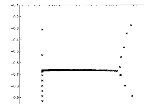
Fig. 1. Eigenvalues of the Orr–Sommerfeld operator (n= 400; = 1; R= 1000):
and second, the Lanczos method for computing the smallest eigenvalue of the Hermitian matrix
−(A22+A∗22)=2.
It is clear that the proposed algorithm works well if the number r of the required rightmost
eigenvalues is not very large.
Let us illustrate the behavior of the algorithm on the Orr–Sommerfeld operator [14] dened by
1
RL
2y
−i(ULy−U′′y)−Ly= 0; (32)
where andR are positive parameters, is a spectral parameter number,U= 1−x2; y is a function
dened on [−1,+1] with y(±1) =y′(
±1) = 0; L= d2=dx2 −2:
Discretizing this operator using the following approximation
xi=−1 + ih; h=
2
n+ 1;
Lh=
1
h2Tridiag(1;−2− 2h2;1);
Uh= diag(1−x12; : : : ;1−x 2
n);
gives rise to the eigenvalue problem
Au=u with A= 1
RLh−iL −1
h (UhLh+ 2In): (33)
Taking = 1; R= 1000; n= 400 yields a complex non Hermitian matrix A (order n= 400;kAk=
160:80) whose spectrum is plotted in Fig. 1.
For comparison purpose, and since the matrix A is not so large, an application of the Matlab
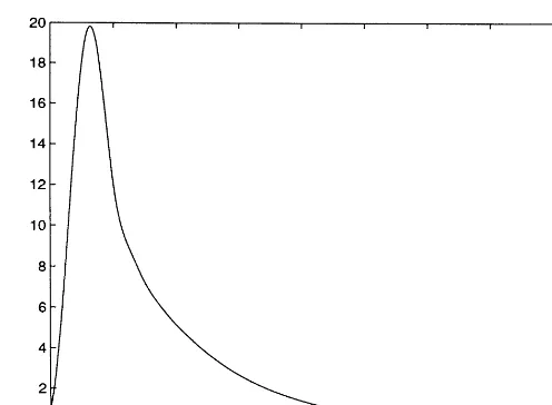
minimization function FMINU to the map ∈R→ k(iI−A)−1k gives rstab(A)≈1:97e−03. Fig. 2
Fig. 2.ket Akvs
: t for the Orr–Sommerfeld operator (n= 400; = 1; R= 1000):
The stability of the Orr–Sommerfeld operator has been studied in [5]. Here we are interested in a simple version of the operator using the above discretization that leads to large matrices.
As we have already mentioned, the approximation of V1 andA11 may be obtained, for example, by
Arnoldi’s method [18]. For the Orr–Sommerfeld example, the basic Arnoldi method was inecient and we had to combine it with complex Chebyshev acceleration techniques [9, 19] which consist in restarting the Arnoldi process using Chebyshev polynomials that amplify the components of the required eigendirections while damping those in the unwanted ones. In this example, we worked with an Arnoldi basis of dimension 40 and Chebyshev polynomials of degree 20. It is clear that other techniques may also be used. We stress that it is not the intention of this note to compare the
eciency of existing sophisticated eigenvalue methods, but rather to show how rstab(A) and ket Ak
may be relatively cheaply approximated.
The computation of is done with the Hermitian Lanczos method which is very suitable for
computing the extreme parts of the spectrum of Hermitian matrices [18].
Using the above algorithm, the condition “A11 stable andA22+A∗22¡0” of Proposition 3.1 occurred
for the rst time when
r= 10 and = 4:91e−02 (34)
with a tolerance
= 1:00e−10 (35)
for both Arnoldi and Lanczos methods.
We applied the Matlab minimization function FMINU to the map ∈R→ k(iI−A11)−1
k and obtained
Several “tricks” can be used to estimate kA12k. The obvious one is kA12k6kAk= 160:80 but we
can notice from (21) or (24) that kA12k6kV1∗Ak= 1:35e + 00. Note that the exact computation of
kA12k gives kA12k= 0:65.
The parameters r1; r2 and r3 of Proposition 3.1 are then:
r1≈1:01e + 04; r2≈9:83e + 03 and r3≈9:81e + 03: (37)
Therefore,
rstab(A)¿1:01e−04−: (38)
The Lyapunov equation A∗11H +HA11+I= 0, solved by the Matlab LYAP function gives
M=qkHkkH−1k= 2:86e + 01 and != 1
2max(H)
= 2:04e−03: (39)
Therefore, inequality (4) of Theorem 2.1 can be written as
ket A11k6Me−! t; t¿0: (40)
From Proposition 3.2, we have
ket A0k6M(1 +tkA
12k) e−! t; t¿0: (41)
and
ket A
k6Ce(−!=2+C)t; t¿0 with C= 3:78e + 04: (42)
5. Conclusion
We have proposed and justied mathematically some techniques for analyzing the stability radius and the behavior of the norm of the exponential of large matrices. The proposed method uses Krylov subspace techniques to split the matrix into two blocks: a rst block corresponding to the rightmost eigenvalues, explicitly given by the Krylov method, in which the stability radius and the norm of the exponential can be estimated using the standard methods, and a second block, whose eld of values, estimated by the Hermitian Lanczos method, must belong to the left-half part of the complex plane. The method should work well if the block corresponding to the rightmost eigenvalues is small. In particular, this technique is suitable for elliptic operators and more generally for sectorial operators [13, p. 280], [6], i.e. operators whose eld of values lies in a sector, provided that the part of the sector which lies on the right-half plane of the complex plane is small.
Acknowledgements
References
[1] A.Ya. Bulgakov, An ecient calculable parameter for the stability property of a system of linear dierential equations with constant coecients, Siberian Math. J. 21 (1980) 339–347.
[2] R. Byers, A bisection method for measuring the distance of a stable to unstable matrices, SIAM J. Sci. Statist. Comput. 5 (1988) 875–881.
[3] G. Dahlquist, Stability and error bounds in the numerical integration of dierential equations, Trans. Royal Institute of Technology, No. 130, Stockholm, Sweden, 1959.
[4] J.L.M. van Dorsselaer, J.F.B.M. Kraaijevanger, M.N. Spijker, Linear stability analysis in the numerical solution of initial value problems, Acta Numerica (1993) 199–237.
[5] P.G. Drazin, W.H. Reid, Hydrodynamic Stability, Cambridge University Press, Cambridge, 1981.
[6] S.K. Godunov, Spectrum dichotomy and stability criterion for sectorial operators, Siberian Math. J. 36 (1995) 1152–1158.
[7] G.H. Golub, C.F. van Loan, Matrix computations, 2nd ed., The Johns Hopkins University Press, Baltimore, 1989. [8] C. He, V. Mehrmann, Stabilization of large linear systems, Tech. Rep., TU Chemnitz–Zwickau, PSF 964, D-09009
Chemnitz, 1994.
[9] V. Heuveline, M. Sadkane, Chebyshev acceleration techniques for large complex non hermitian eigenvalue problems, Reliable Computing 2 (1996) 111–119.
[10] D. Hinrichsen, A.J. Pritchard, Stability radii of linear systems, Systems Control Lett. 7 (1986) 1–10. [11] R.A. Horn, C.R. Johnson, Topics in Matrix Analysis, Cambridge University Press, Cambridge, 1991. [12] B. Kagstrom, Bounds and perturbation bounds for matrix exponential, BIT 17 (1977) 39–57. [13] T. Kato, Perturbation Theory for Linear Operators, Springer, Berlin, 1976.
[14] W. Kerner, Large-scale complex eigenvalue problems, J. Comp. Phys. 85 (1989) 1–85.
[15] R.J. LeVeque, L.N. Trefethen, On the resolvent condition in the Kreiss matrix theorem, BIT 24 (1984) 584 –591. [16] C.F. van Loan, The sensitivity of the matrix exponential, SIAM J. Numer. Anal 14 (1977) 971–981.
[17] C.F. van Loan, How near is a stable matrix to an unstable matrix, Contemporary Math. 47 (1985) 465– 478. [18] Y. Saad, Numerical methods for large eigenvalue problems, Algorithms and Architectures for Advanced Scientic
Computing. Manchester University Press, Manchester, UK, 1992.
[19] M. Sadkane, A block Arnoldi-Chebyshev method for computing the leading eigenpairs of large sparse unsymmetric matrices, Numer. Math. 64 (1993) 181–193.