www.elsevier.comrlocatereconbase
Horizon sensitivity of the inflation hedge of
stocks
Peter C. Schotman
a,), Mark Schweitzer
ba
Limburg Institute of Financial Economics and Global Property Research, Maastricht UniÕersity, PO Box 616, 6200 MD Maastricht, Netherlands
b
Limburg Institute of Financial Economics and CEPR, Maastricht UniÕersity, PO Box 616, 6200 MD Maastricht, Netherlands
Abstract
In this paper, we study the potential of stocks as a hedge against inflation for different investment horizons. We show that stocks can be a hedge against inflation even if stock returns are negatively correlated with unexpected inflation shocks, and only moderately positively related to expected inflation. Depending on the investment horizon, the optimal hedge ratio can be either positive or negative. The crucial parameter for the results is the persistence of inflation.q2000 Elsevier Science B.V. All rights reserved.
JEL classification: E31; E44; G11; G23
Keywords: Stock returns; Inflation; Hedge ratio; Risk management
1. Introduction
One of the biggest fears for investors is increasing inflation, because it reduces the real return on investments. As with any other risk in the financial market, the investor might want to try to reduce the risk exposure by adjusting the composi-tion of the portfolio.
)
Corresponding author. Tel.:q31-43-388-3862; fax:q31-43-388-4875.
Ž .
E-mail address: [email protected] P.C. Schotman .
0927-5398r00r$ - see front matterq2000 Elsevier Science B.V. All rights reserved.
Ž .
In this paper, we focus on the risk associated with inflation and the extent to which stocks can be used as a hedge against inflation. The theoretical basis for this strand of the literature is the Fisher hypothesis, describing the link between real and nominal returns. Applied to stocks, the Fisher hypothesis implies that there should be a one-to-one relation between expected nominal stock returns and expected inflation. However, in contrast to the Fisher hypothesis, many empirical studies observed a negative relation between inflation and stock returns.1 It seems,
however, that there is an important horizon effect. More recent studies find a positive relation at a horizon of 5 years or longer.2 In this paper, we focus on the
hedge potential and examine how it is influenced by the investment horizon. An explanation for the short-term negative hedge potential of stocks is offered
Ž .
by Fama 1981 , who argues that inflation simply acts as a proxy for real-activity variables in relations between inflation and stock returns. Higher expected eco-nomic activity would lead to an increase in stock returns, but due to the short-term non-neutrality of money, increasing inflation leads to lower economic activity and thus to lower stock returns.
In contrast to this negative effect, one would expect the Fisher hypothesis to
Ž .
hold in the long run. For example, Campbell and Shiller 1988 explain that inflation has two effects in a present value relation linking the stock price to the expected discounted future dividends. First, higher inflation increases the discount rates, which lowers returns. The second effect of increasing inflation is the rise of future dividends and therefore the rise of expected stock returns. Due to nominal price rigidities in the short run, the price elasticity of future cashflows is not necessarily equal to one. This means that the net effect is ambiguous in the short run, but will be positive in the long run.
Time series characteristics are important when we explore the horizon sensitiv-ity. First, the volatility of stock returns is usually much higher than the volatility of inflation, which makes it difficult to test for correlation between stock returns and inflation. Even more important is the widely recognized strong persistence of inflation, probably related to inertia of monetary policies carried out by the central banks.
The horizon sensitivity is very important for investors who have to deal with inflation risk. An investor might not be interested in short-term performance at all. Institutional investors like pension funds have a very long horizon. Under a defined benefit plan, they often have inflation-linked liabilities with a duration of 15 years or more. It is therefore interesting to study the effects of changing correlation coefficients when the investment horizon increases. The changing
1 Ž . Ž . Ž .
See, for example, Fisher 1930 , Bodie 1976 , Fama 1975, 1981, 1990 , Fama and Schwert
Ž1977 , Geske and Roll 1983 , James et al. 1985 , and Lee 1992 who all reject the Fisher hypothesis. Ž . Ž . Ž .
and indicate that stocks are a poor hedge against inflation.
2 Ž . Ž .
covariance structure of stocks and inflation will affect the hedge potential of stocks. Horizon effects could lead to stocks being a poor hedge against inflation in the short run, but implying a positive long-run hedge ratio.
In this paper, we examine the portfolio problem of a long-term investor who faces inflation risk. We develop a model that accommodates the two following stylized facts: a short-term negative hedge ratio and long-term positive hedge ratio. The remainder of the paper is organized as follows. In Section 2, we set up the theoretical model. In Section 3, we discuss parameter values for the model. In Section 4, we present the results. In Section 5, we discuss the relations with other literature and in Section 6, we conclude.
2. The long-term inflation hedge potential of stocks
In this section, we use a stylized model of stock returns to explain how the hedge ratio will change with the investment horizon. We assume that the one-period stock return is generated by:
w
x
Rtq1scqbEt ptq1 qfhtq1qetq1
Ž .
1The stock return Rtq1, which has a constant part c, depends on the expected
w x
inflation Etptq1, unexpected inflation htq1, and a specific risk term etq1 with mean zero and variances2
. The strength of the Fisher relation is represented by
e
b, which measures the relation between expected inflation and stock returns. If b
is equal to 1, the Fisher hypothesis holds, and expected real returns are constant. The coefficient f is theAinflation betaBof stocks and indicates how stock prices adjust instantaneously to unexpected inflation.
Ž .
Inflation is assumed to be generated by the AR 1 process
ptq1smqa p
Ž
tym.
qhtq1Ž .
2 Current inflation depends on the long-run inflation m, the deviation of inflation in the previous period from the long-term mean, and an independent shock ht with variance s2. The inflation process could be augmented by additional transitoryh
Ž .
noise terms, but for transparency reasons, we decided to use this AR 1 model
Ž .
with inflation persistence a as the key parameter. When inflation is an AR 1
Ž .
process, the expected stocks returns are also AR 1 , and actual stocks returns are
Ž . Ž .
ARMA 1,1 . Campbell et al. 1997, Chap. 7 argue that such dynamics are
empirically relevant for US stock returns. In the limiting caseas1, both inflation and stock returns have a unit root. However, when s2
is much smaller than s2
,
h e
stock returns will still be almost unpredictable over short horizons. In addition, in short samples, the slow but persistent movements in expected returns will hardly be visibly relative to the noise of et. This is a reason why econometric inference
Ž .
on b in Eq. 1 is problematical in short samples.
Ž .
in stocks, and 1yw is invested in a nominally risk-free discount bond of
maturity k. The maturity of the bond equals the horizon of the investor. The goal of the investor is to maximise the mean–variance criterium
Žk. cumulative nominal stock return, pŽk. the cumulative inflation, RŽk. the
nomi-tqk f, t
nally risk-free cumulative return on a discount bond with maturity k, and g the risk tolerance parameter. The investor solves a single-period optimization problem, but the covariance matrix of asset returns and inflation changes with the investor
Ž .
horizon. As argued in Canner et al. 1997 , this provides a tractable way to incorporate asset price dynamics. The solution of the portfolio problem is
Žk. Žk. Žk. Žk.
gE RtqkyRf , t cov Rtqk,ptqk
Žk.
w s Žk. q Žk.
Ž .
4var Rtqk var Rtqk
The first term is the demand for stocks as a result of the equity premium. The second term is the hedging demand for stocks depending on the covariance with inflation. It is this second component of the portfolio demand that we will focus on. The hedging demand will be denoted DŽk.
.
Ž
For the one-period model, the hedge ratio is see Appendix A and also Bodie
Ž1976 :..
Eq. 5 shows that the negative value of f immediately implies a negative hedge
Ž .
ratio. For the single-period hedge in Eq. 5 , the Fisher coefficientb does not play a role at all.
We continue with a two-period model, in which we define the two-period return RŽ2.
as the sum of the return in the first period plus the return in the tq2
second period.3 For the two-period return, we obtain
Ž2. Ž2.
w
x
Rtq2sbEt ptq2 qb
Ž
Etq1yEt.
ptq2 qf hŽ
tq1qhtq2.
qetq1qetq2
Ž .
6In the two-period model, the unexpected rise in inflationhtq1 has two effects. The direct effect is fhtq1, which is the same as in the one-period model. The indirect
3
Ž .w x
effect b Etq1yEt ptq2 is due to the adjustment of inflation expectations. An unexpected shock htq1 will lead to an upward revision in expected inflation of
ahtq1 and higher expected return bahtq1. The total effect depends on the sign
Ž .
and size of fqab . At the same time, the new shockhtq2 only has a negative effect on the hedge potential.
If we extend our model to a multi-period setting, the Fisher coefficient becomes more important at the expense of the short-term effect. Since we assume that inflation is persistent, a shock this year has an effect on all future periods. The higher the persistence, the more the expectation revisions accumulate. In Appendix A, the hedge ratio for any horizon k is derived. The result is stated in Proposition 1:
Proposition 1. Assume that stock returns and inflation are generated by the
( ) ( ) < <
The hedge ratio is a complicated function of all parameters in the model. The limit as k™`is:
which reduces to 1rb for as1. The long-run hedge ratio will be positive if
1ya fqab)0 10
Ž
.
Ž
.
Ž .
The hedge demand for stocks can be large relative to the demand due to the equity premium. The infinite horizon portfolio weight from solving the mean–
Ž Ž ..
premium. Due to the factor 1-a , the expected return becomes rapidly less
influential, the higher the inflation persistence a. If as1, the only long-run demand for stocks is the hedging demand, whatever the expected returns.
3. Parameter estimates
To illustrate the hedging potential of stocks in the model, we use benchmark
parameters found in the literature. The parameters a, b and f have been
estimated for many different countries, sample periods and observation frequen-cies.
The starting point for empirical results for the inflation hedge regression model
ŽEq. 1Ž ..are the studies of Bodie 1976 and Fama and Schwert 1977 . AccordingŽ . Ž .
to their empirical evidencef is almost certainly negative. The Fisher parameter b
Ž .
could also be negative, but is estimated without much precision. Bodie 1976 can
Ž .
reject neither the hypothesisbs1 norbs0. Fama and Schwert 1977 , however, find that b is significantly negative for US data for the period 1953–1971, using a short-term interest rate as a proxy for expected inflation. For the inflationAbetaB
Ž
their most reliable estimate isfs y4 for quarterly data. With monthly or higher
. Ž .
frequency data Schwert 1981 shows that measurement of f is troublesome due
to the announcement effects. The official announcement of monthly inflation occurs with a lag of almost 1 month, but some news about inflation seems to
AleakB to the market before the announcement date.
Ž .
Using quarterly data for 16 countries between 1957 and 1990, Beckers 1991 provides an update of the evidence. Inflation is separated in expected and unexpected components by assuming that inflation follows a random walk plus noise process. The immediate inflation risk f is significantly negative for five
countries, and ranges between y3 for the US to q1.5 for Finland, with an
average ofy0.75. Although point estimates for b are consistently negative, it is significantly negative for only three countries.
The problem with the estimation of b is that the time series properties of
dependent variable and independent variables in the regression are very different. Stock returns are very noisy, whereas expected inflation is a slowly moving
Žalmost nonstationary series. Furthermore, expected and unexpected inflation are.
series model for inflation. Misspecification in this model or instability of the parameters leads to measurement errors.
The measurement error can be avoided by using total inflation instead of its components in the regresssion. When inflation is close to being nonstationary, a regression of cumulative stock returns over k periods on cumulative inflation over the same horizon would give an estimate of b if k gets large enough. This is the
Ž .
approach taken by Boudoukh and Richardson 1993 . Using OLS estimates based on 200 years of US data they find a significant positive coefficient of around 0.5 at 5-year horizons. For instrumental regression, the estimates of the effect of
Ž .
expected inflation b range between 0.7 and 2.0 at the 5-year horizon depending
Ž .
on the instrumental variables used to predict inflation. Lothian and Simaan 1998
Ž .
and Solnik and Solnik 1997 corroborate the findings of Boudoukh and
Richard-Ž .
son 1993 using panel data for a shorter period.
Another way of measuring expected inflation is the use of survey data. For
Ž .
example, with quarterly survey data on US inflation expectations Sharpe 1999 finds that Aa one percentage point increase in expected inflation is estimated to raise required real stock returns about a percentage point, which amounts to about
Ž Ž ..
a 20% decline in stock prices.B In terms of the stock return model Eq. 1 , this
means that bs2 and fs y20.
The latter estimate follows from a present value calculation discussed in detail
Ž .
in Campbell et al. 1997, Chap. 7 . A small increase in the expected return raises the rate at which future cashflows are discounted. The more persistent the shock to the expected return process, the larger the effect of an increase in the expected return on all future discount rates. The parameterf measures the total decrease in
Ž .
the present value resulting from such a shock. For example, if as1 and bs1 , then f should be approximately y24. This present-value implied effect is much
Ž .
larger than what is obtained from the regression estimates of f based on Eq. 1 . The reason is that the inflation hedge regression does not distinguish between temporary and persistent shocks to inflation. Not all unexpected inflation has a
Ž .
persistent effect on future expected inflation, but in Eq. 1 , they are lumped
together.4 Since the magnitude of f depends on the inflation persistence, we
would expect that f can differ across countries if differences in monetary policy lead to differences in the inflation process.
The relation betweenf and inflation persistence naturally leads to the literature on estimating the persistence of inflation. The empirical literature reports a lot of uncertainty around the parametera. Some studies find that as1, others find that the process has changed between the seventies, eighties and nineties, and the
4
For example, lethtsh1 tqh2 t, whereh1 is the persistent shock to expected inflation andh2 is a pure transitory shock. Assume thath and h are uncorrelated and have variances s2s0.5 and
1 2 1
s2s3.5. Let the impact on stock returns of both shocks be given asf sy20 andf sy1. If only
2 1 2
Ž . Ž 2 2. Ž 2 2.
htq1 is used in Eq. 1 instead of its two components, thenfsf s1 1qf s2 2 rs1qs2 sy4.3.
Ž . Ž .
Table 1 Parameter values
Parameter a b f sh se
w x Ž x
Value 0.7, 1 0, 2 y4 2% 20%
The entries give the parameter inputs for the hedge ratio computations in Section 4. The numbers refer to annual data. Fora and b, different values within the indicated range will be used.
process seems to differ between the EU countries and the US. Some references to
Ž .
the voluminous empirical literature on inflation dynamics are Barsky 1987 ,
Ž . Ž . Ž .
Juselius 1995 , Haldrup 1998 , Hassler and Wolters 1995 , Evans and Lewis
Ž1995 and Fuhrer and Moore 1995 .. Ž .
The variances of the unexpected changes of the stock returns and inflation are also important. In fact, it is only the ratio sersh that matters. The stylized facts about stocks returns and inflation are discussed in several sources. For example, in
Ž .
Table 1-1 of Siegel 1998 , the volatility of real annual stock returns in the US for
Ž .
the 20th century is 20%. Bodie et al. 1999, Chap. 5 find similar numbers. A recent estimate of the volatility of 1 year ahead unexpected inflation is in Table 1
Ž .
of Thomas 1999 , who puts it at 2% for the period since 1960. In the hedge ratio computations, we will use shs2.0% and ses20.0%, both on an annual basis. Since se4sh, the conditional variance of one-period stock returns will be almost entirely determined bys2. On the other hand, the unconditional variance of stock
e
returns could be dominated by the unconditional inflation variance if the inflation persistence is large enough. This creates the difference between short-term and long-term hedge ratios.
Table 1 summarises the parameter values that will be used to illustrate the
Ž .
quantitative properties of the hedge ratio implied by Eq. 7 . As most of the uncertainty is in the parameters a and b, the results will be presented for several different values of these parameters.
4. Results
Ž Ž ..
Since the one period hedge ratio Eq. 5 does not depend on a and b, we can
substitute the numbers forf,sh and se in the first line of Table 1 to get a hedge ratio ofy2%, which means that the investor should short 2% of the portfolio in stocks to have the optimal protection against inflation with a 1-year investment horizon.
Table 2 presents the infinite horizon hedge ratio for different values of the inflation persistence and the coefficient for the Fisher hypothesis. If there is little
Ž .
Table 2
Long-term hedge ratios
b a
0.70 0.90 0.95 1
0 y0.11 y0.34 y0.69 y`
0.7 y0.07 0.22 1.00 1.43
1.0 y0.05 0.40 0.92 1
2.0 0.02 0.47 0.54 0.50
The entries show the infinite horizon hedge ratios for different values ofa and b. Other parameter values:fsy4,shs2% andses20%. Parameter values are based on annual data.
With higher inflation persistence the hedge potential depends strongly on the Fisher coefficient b. When the Fisher hypothesis holds and inflation is a random walk, stocks are a perfect long-term hedge and an investor with infinite horizon should invest all her wealth in stocks. If the Fisher hypothesis does not hold at all
Žbs0 , the infinite horizon hedge ratio diverges to minus infinity, which is.
consistent with the model, but not very realistic. This result obtains, since the variance of inflation risk goes to infinity when inflation is an integrated process. In the absence of the Fisher effect, nominal stock returns do not offer any expected compensation for this infinite risk. On the contrary, stocks will be hit by every new inflation shock through fht, and are therefore very unattractive. In the intermediate case that bs0.7, the infinite horizon hedge ratio is larger than under the full Fisher hypothesis.
The relation between b and the hedge ratio is not monotonically increasing in
b. In the extreme case that as1, the hedge ratio is 1rb and inversely related to
b. For a slightly less than 1, the infinite horizon hedge ratio is first positively related to b, but starts declining for large values of b.5
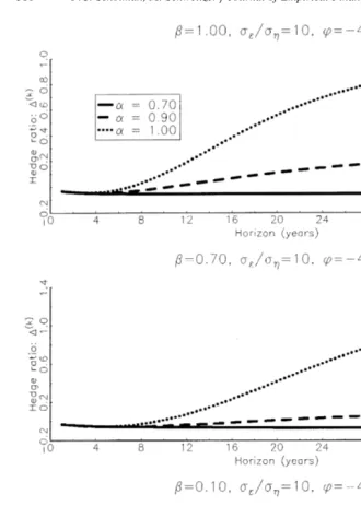
The intermediate hedge ratios implied by the model can be very different from either the single-period or the infinite horizon hedge ratios. Fig. 1 presents graphs of the hedge ratio against the investment horizon for different parameter combina-tions of a and b. The 1-year horizon with DŽ1.
s y0.02 is the starting point for
Ž .
all lines in Fig. 1. As shown in Eq. 5 , this point is independent of both a and b. When both b and a are equal to 1, the hedge ratio is first negative, but starts to increase from the 5-year horizon and becomes positive at the 8-year horizon, from which it quickly rises to the long-run value of unity. For lower values of a, the hedge ratio increases later, less quickly and to a lower value. For as0.7, the hedge potential is negligible at all horizons.
Ž .
When the Fisher hypothesis only holds partly bs0.7 , we see a similar
picture in the second panel of Fig. 1. If inflation is persistent, the hedge ratio will
5 Ž Ž ..
Differentiating the infinite horizon hedge ratio formula Eq. 9 with respect to b, it follows that
Ž .Ž 2 2. 2
Fig. 1. Hedge ratios for different values of a and b. The figure shows the hedge demand for stocks
DŽk.for investors with invesment horizon k years using the parameters in Table 1.
today’s inflation shocks have only a direct effect on the stock return and not much on tomorrow’s inflation.
When b is small, Fig. 1 shows that the hedge ratio is still negative at the 40-year horizon, regardless of inflation persistence. Even with persistent inflation, the convergence to its long-run value of 1rbs10 is terribly slow.
Summarising, stocks provide a hedge against inflation if the investor horizon is
Ž .
longer than 15 years, and the investor believes that inflation is persistent aG0.9 and there is at least a partial feedback from expected inflation to expected nominal
Ž .
stock returns bs0.7 .
5. Discussion
The previous section showed that stocks have a hedge potential over longer investment horizons. It also showed how the hedge potential depends on key parameters like inflation persistence, the Fisher effect, and the inflation beta of stocks. In this section, we discuss a number of further issues and related work on the hedge potential of stocks.
The weight of stocks in the optimal portfolio is based on the assumption that the remaining part of the portfolio is invested in an asset that pays a fixed nominal amount at the end of the investment horizon. In practice, investors can choose between many different asset categories that each have their own hedge potential. For example, in our model, the long-term risk-free asset is not a hedge against inflation at all, since nominal terms are fixed and real returns are dependent on the realized inflation. With the existence of a short-term nominally risk-free asset investors could choose to roll over short-term bonds. Whether this provides a better hedge against inflation depends on the relation between the short-term interest rate and inflation. The empirical literature on the Fisher hypothesis for interest rates is even more voluminous than for equity returns, and the general conclusion is that real interest rates are negatively related to inflation in the short run, but positively in the long run, and that real interest rates are moderately persistent.6 The implications for an optimal portfolio of equity, short-term bonds and long-term bonds are not clear a priori.
Ž .
Some answers can be found in Campbell and Viceira 2000 . Campbell and
Ž .
Viceira 2000 consider an infinitely lived investor who can choose from an asset menu consisting of nominal and real, both long and short, bonds and equity. They
Ž .
derive explicit solutions for the Merton 1973 intertemporal hedging demand for each asset category, and find that both long-term bonds and equity play a role in
6 Ž . Ž . Ž .
A few references are Fama and Schwert 1977 , Mishkin 1992 , Evans and Lewis 1995 and
Ž .
the hedge portfolio, with nominal bonds becoming more important the higher the
Ž .
risk aversion. Campbell and Viceira 2000 assume, however, that bs1 for all
assets. The Fisher hypothesis holds for expected returns, although it does not need to hold for the unexpected returns, and f also differs over asset classes.7
As shown, the hedge ratios can be very sensitive to the parameter values forb,
f and a. For some values of the parameters, stocks offer a strong hedge against inflation, for other values, the hedge potential is close to zero. To arrive at an overall estimate, one should take the parameter uncertainty into account. A straightforward exercise would be to estimate the standard error of the hedge ratio
DŽk.
as a function of the parameters of the model. For a rough calculation, assume each of the nine scenarios in Fig. 1 as equally likely. This assumption is in line with the range of estimates fora and b encountered in the literature. In that case, the average over these nine scenarios gives a positive value for horizons longer than 15 years. However, the dispersion increases rapidly with the horizon. The long-run hedge ratio is positive for four scenarios, and negative for the other five.
6. Conclusion
This paper showed that the negative inflation hedge potential of stocks can become positive if the investment horizon changes. In the model, a short-term negative sign is consistent with the positive hedge ratio implied by the Fisher hypothesis in the long run. The crucial parameter is inflation persistence. The higher the inflation persistence, the better the performance of stocks as a hedge against inflation. Even if the Fisher coefficient is only slightly positive, the inflation persistence still causes a positive inflation hedge of stocks at longer horizons. This horizon effect can be important for investors that have a long-run perspective.
Acknowledgements
We would like to thank Casper De Vries, Clemens Kool, Christian Wolff,
Ž .
Franz Palm the editor and participants at the 1998 ESEM in Berlin and the JEF-LIFE conference on risk management for valuable comments. All errors remain the responsibility of the authors.
7 Ž .
To be precise, from Table 1 of Campbell and Viceira 2000 , one can deduce thatfsy2.25 for
Ž . Ž
stocks on quarterly data . The effective horizon in their model is about 25 years duration of a constant
.
Appendix A. Derivation of the hedge ratios
This appendix provides a derivation of the long-term hedge ratios in Proposi-tion 1. As a VAR, the model is written
xtq1sF xtqG etq1
Ž
12.
Ž .X Ž .X
where xts Rt pt contains the stock return and inflation, ets e ht t is the vector of mutually uncorrelated shocks, and the matrices F and G are defined as
0 ab 1 f
Fs
ž
/
and Gsž /
0 a 0 1
The covariance matrix of the shocks is
s2
qf2s2 fs2
e h h
V'Var G e
Ž
t.
sž
fs2 s2/
Ž
13.
h h
A first step in the derivation of the hedge ratio is the conditional covariance matrix of returns and inflation for every horizon k. Define
k Žk.
ytqks
Ý
xtqjjs1
as the k-period return vector. Its conditional covariance matrix is given by X
From this, the k-period hedge ratio is directly given by
VŽk.
To provide analytical detail on the properties of the hedge ratio, we explicitly compute the long-run covariance matrix as a function of the underlying structural parameters. The powers of F are found as
Calculating the covariance matrix fora/1 gives:
Using the covariance matrix Eq. 17 , the hedge ratio follows as given in
Proposition 1.
The limiting behavior of the covariance matrix when inflation is a random walk is determined by the limit as a™1. It is easier to recalculate the covariance
Ž . Ž .
which leads to Eq. 8 in Proposition 1.
References
Barsky, R.B., 1987. The fisher hypothesis and the forecastability and persistence of inflation. Journal of Monetary Economics 19, 3–24.
Beckers, S., 1991. Stocks, bonds, and inflation in world markets: implications for pension fund investment. Journal of Fixed Income, 18–30, Dec.
Boudoukh, J., Richardson, M., 1993. Stock returns and inflation: a long horizon perspective. American Economic Review 83, 1346–1355.
Campbell, J.Y., Lo, A.W., MacKinlay, A.C., 1997. The Econometrics of Financial Markets. Princeton Univ. Press, Princeton.
Campbell, J.Y., Shiller, R.J., 1988. Stock prices, earnings and expected dividends. Journal of Finance 43, 661–676.
Campbell, J.Y., Viceira, L.M., 2000. Who Should Buy Long-Term Bonds? American Economic Review, forthcoming.
Canner, N., Mankiw, N.G., Weil, D.N., 1997. An asset allocation puzzle. American Economic Review 87, 181–191.
Crowder, W.J., Hoffman, D.L., 1992. The long-run relationship between nominal interest rates and inflation: the fisher equation revisited. Journal of Money Credit and Banking 28, 102–118. Evans, M.D.D., Lewis, K.K., 1995. Do expected shifts in inflation affect estimates of the long-run
fisher relation. Journal of Finance 50, 225–253.
Fama, E.F., 1975. Short term interest rates as predictors of inflation. American Economic Review 65, 269–282.
Fama, E.F., 1981. Stock returns, real activity, and money. American Economic Review 71, 545–565. Fama, E.F., 1990. Stock returns, expected returns, and real activity. Journal of Finance 45, 1089–1108. Fama, E.F., Schwert, G.W., 1977. Asset returns and inflation. Journal of Financial Economics 5,
115–146.
Fisher, I., 1930. The Theory of Interest. Macmillan, NY.
Fuhrer, F., Moore, G., 1995. Inflation persistence, quarterly. Journal of Economics 110, 127–159. Geske, R., Roll, R., 1983. The fiscal and monetary linkages between stock returns and inflation.
Journal of Finance 38, 1–33.
Ž .
Haldrup, N., 1998. An econometric analysis of I 2 variables. Journal of Economic Surveys 12, 595–650.
Hassler, U., Wolters, J., 1995. Long memory in inflation rates: international evidence. Journal of Economics and Business Statistics 13, 37–45.
James, C., Koreisha, S., Partch, M., 1985. A Varma analysis of the causal relations among stock returns, real output, and nominal interest rates. Journal of Finance 40, 1375–1384.
Juselius, K., 1995. Do purchasing power parity and uncovered interest parity hold in the long run? Journal of Econometrics 69, 211–240.
Lee, B., 1992. Causal relations among stock returns, interest rates, real activity, and inflation. Journal of Finance 42, 1591–1603.
Lothian, J.R., Simaan, Y., 1998. International finance relations under the current float: evidence from panel data. Open Economics Review 9, 293–313.
Merton, R.C., 1973. An international capital asset pricing model. Econometrica 41, 867–889. Mishkin, F.S., 1992. Is the fisher effect for real? Journal of Monetary Economics 30, 195–215. Schwert, G.W., 1981. The adjustment of stock prices to information about inflation. Journal of Finance
36, 15–29.
Siegel, J.J., 1998. Stocks for the Long Run. 2nd edn. McGraw-Hill, NY.
Solnik, B., Solnik, V., 1997. A Multi-Country Test of the Fisher Model for Stock Returns. Journal of International.