Energy Use By Apartment Tenants When Landlords Pay For Utilities
February 2003
Arik Levinson
Georgetown University and NBER
Scott Niemann Charles River Associates
Abstract
Energy costs are included in the monthly rent of more than one-fourth of U.S. apartment
residents. Because these tenants do not face the marginal cost of their own energy use, they have little incentive to use energy efficiently. Explanations for this apparent market failure fall into two categories: the tenants value such arrangements more than they value the extra energy they consume, or the landlords value the arrangements more than the cost of that extra energy. We use data from the U.S. Department of Energy's Residential Energy Consumption Survey and the Census Bureau's American Housing Survey to estimate energy consumption by tenants in included apartments, and the rent premium for those apartments. While market rents for utility-included apartments are higher than for otherwise similar metered apartments, the difference is smaller than the cost of the energy used, a finding that supports landlord-side explanations.
Key Words: energy efficiency, average-cost pricing, utilities
JEL Codes: Q4, L85, L97
Acknowledgments
Introduction
More than one-fourth of rental apartments in the U.S. have the cost of utilities included in
their rent. Because tenants in these apartments choose how much energy to use after the monthly
rent has been determined, they have no price incentive to conserve energy, and therefore use
more energy than tenants in otherwise similar individually metered apartments. Moreover, the
cost of the extra energy use, if added to tenants' monthly rent, will be more than tenants would be
willing to pay for that energy separately. Tenants or landlords, or both, must be worse-off under
utility-included contracts than with individual metering. The existence of these utility-included
contracts therefore raises two questions that we address in this paper: (1) how much extra energy
is used by tenants in these apartments, and (2) what explains the persistence of this seemingly
inefficient institution.
The obvious explanation for the apparent inefficiency, that retrofitting old buildings and
individual metering are costly, cannot be the entire story. Many newly built, electrically heated
apartments include utilities in their rents. Explanations in addition to metering costs must
account for some of the utility-included rental contracts: economies of scale in master-metering,
signaling costs associated with investments in energy efficiency, risk-averse or liquidity
constrained tenants, or tenants who simply dislike considering marginal costs. We discuss each
of these explanations below.
Beyond academic curiosity, a number of important policy concerns hinge on the answer
1Authors' calculations using data for 1997 from the 1999 Energy Information Agency's Annual Energy Outlook, U.S. Department of Energy, Washington DC.
2PURPA did not, however, prohibit utility-included rental contracts, and some new, individually metered, electrically heated apartments are rented with utilities included. See Munley,et al.(1990).
31998 Code of Federal Regulations, Title X, part 435.106.
4See for example, Hausmann (1979), Jaffe and Stavins (1994), and Hassett and Metcalf (1995, 1999).
Residential and commercial buildings account for about 35 percent of U.S. energy consumption,1
and the energy sector is one of the largest contributors to national and global environmental
problems. Each of the potential explanations for the persistence of utility-included rental
contracts has its own set of welfare implications and policy prescriptions.
For example, the Public Utilities Regulatory Policy Act of 1978 (PURPA) required newly
constructed apartments to be individually metered for electricity.2 Similarly, federal energy
efficiency guidelines encourage individual metering for residential buildings: "Tenant
submetering can be one of the most cost-effective energy conservation measures available. A
large portion of the energy use in tenant facilities occurs simply because there is no economic
incentive to conserve."3 If, however, landlords with utility-included contracts invest in more
energy efficient construction and appliances, a ban on such contracts mayincreaseenergy
consumption, and decrease welfare.
Another policy implication involves the so-called "energy paradox" -- the surprisingly
slow adoption of cost-effective residential energy-conservation technologies.4 Common
discount rates, and liquidity constraints. This paper describes what may be another important
explanation for the slow adoption: rental contracts with zero-marginal-cost energy use.
Finally, because energy is heavily regulated, some have suggested that "win-win" policies
would both increase measured economic welfare and reduce pollution. Utility-included rental
contracts seem a likely source of such win-win policies. If some market failure, policy-induced
or otherwise, underlies the utility-included rents, then correcting that market failure may increase
economic welfare while reducing energy consumption and pollution.
In what follows, we use data on apartment rental configurations and utility use to examine
competing explanations for utility-included rents. We first assess the scale of the deadweight
loss from utility-included apartments by estimating how much more energy their tenants use,
after controlling for self-selection by individuals and landlords. Then we estimate rent
differentials between utility-included and metered apartments, controlling for other observable
apartment characteristics. The difference in rent, when compared to the difference in energy use,
sheds light on the potential explanations for the existence of these utility-included rental
contracts.
In brief, we find that tenants living in utility-included apartments set their thermostats
between one and three degrees (Fo) warmer during winter months when they are absent from the
premises, all else equal. This temperature difference translates into approximately half to
three-quarters of a percent increase in fuel expenditures. While the increase in fuel costs is small, there
are several reasons to believe it may be an underestimate. Moreover, given the size of the rental
housing market, even a tiny increase in fuel use amounts to a considerable absolute increase.
significantly less than even this small cost of the extra fuel use, and argue that this outcome
points to landlord-side explanations for the heat-included rental contracts.
Deadweight loss and explanations for utility-included apartments
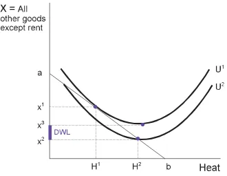
Figure 1 depicts one tenant's consumption choices between heat,H, and all other goods
except rent,X. The tenant's indifference curves are U-shaped because heat becomes undesirable
beyond a satiation point, represented by the minimum point on each curve. Lineabrepresents
the tenant's budget constraint, excluding rent costs, where the tenant pays his own utility bill, and
the price of heat isa/b. A utility-maximizing tenant will chooseH1
units of heat andx1
other
goods, spending (a-x1
) on heat.
Now suppose the landlord includes heat in the monthly rent. Since the tenant faces zero
marginal costs for heating, he will consume heat to the satiation point, the minimum of some
indifference curve. If the landlord is to break even, the monthly rent must increase by enough to
cover the utility bill. This in turn means that the consumption bundle chosen by the tenant must
lie on his original budget line. Point (H2
,x2
) in figure 1 satisfies this condition, resulting in a rent
increase of (a-x2
), an increase in combined housing and heating costs to the tenant of (x1-x2
), and
a lower level of utilityU2
. The compensating variation, the amount the tenant would be willing
to pay to have heat included in his rent is (a-x3
), but the increased costs to the landlord are (a-x2
).
The difference, (x3-x2
), represents the deadweight loss of the inefficient rental contract.
In a perfectly competitive market, with unconstrained credit, economically rational, fully
informed, risk-neutral tenants and landlords, and costless metering of energy use, landlords
willing to pay (a-x3). There would be no reason for landlords to include energy use in rents. To
do so, they would have to charge more additional rent than tenants would be willing to pay.
However, about 30 percent of apartments in the U.S. are rented with utilities included.
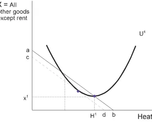
Explanations for the existence of utility-included apartments fall into two categories. The
first is that landlords face some cost of charging tenants for their energy use, the most obvious of
which would be metering costs. In large or older buildings, with one heat source serving
multiple apartments, it may be costly to meter individual units. If metering costs are high
enough, landlords may simply choose to include average expected utility costs in their rent
calculations. Buildings with high metering costs will rent apartments with utilities included, and
buildings with low metering costs will rent apartments with utilities not included. Furthermore,
since tenants presumably do not care about metering costs, they will be borne by landlords in the
form of rent differentials that do not cover the energy expenditures.
Figure 2 depicts a tenant in an unmetered apartment, consumingH1and paying (a-x1
) in
extra rent to cover the utility bill. The tenant would be willing to pay as much as (a-c) in extra
base rent to have an individually metered apartment. If the metering costs are higher than (a-c),
the landlord will not benefit from converting to individual meters. If the metering costs are less
than (a-c), the landlord can meter the apartment individually, pass the cost of doing so on to the
tenant, and pocket the difference. In either case, the rent difference between metered and
heat-included apartments will be less than (a-x1
), the observed cost of the utilities consumed.
Though the metering cost story may be the most obvious explanation for utility-included
apartments, it is not the only explanation. Munley,et al. (1990) present experimental evidence
cost-effective to retrofit many existing master-metered buildings. Furthermore, our calculations using
the Residential Energy Consumption Survey find that many newly constructed, electrically
heated apartments include heat in their rents. Eleven percent of apartments with electric heat in
1993 had heat included, as did 8 percent of apartment buildings less that 15 years old. Because
these buildings, with an easily metered heat source, built since the energy crises of the 1970s,
include heat in their rents, we believe that other explanations account for at least some of the
persistence of utility-included rental contracts.
A second explanation, similar to metering costs, is that there may be economies of scale
in master-metered apartment buildings. Suppose that apartments can be individually metered,
with marginal cost of heata/b, as in figure 3. Tenants will consumeH1
units of heat at cost( a-x1
). Suppose further that a cheaper energy source is available, for fixed cost(a-c), but that this alternative cannot be individually metered, and so rental contracts must include unlimited energy.
(Think of steam heat from a central boiler.) The most a tenant will be willing to pay for such a
contract is (a-x2
), the compensating variation of moving from budget lineabto one with free
heat. The landlord needs to charge only (a-x3
) more rent in order to break even. The difference,
(x3-x2
) represents the gain from moving to a cheaper heat source that cannot be metered
individually.
A final landlord-side explanation rests on asymmetric information. Landlords know the
energy efficiency of their apartments, while prospective tenants do not. Landlords would like to
convey that information credibly to prospective tenants, so that they can charge higher rent and
recoup their energy efficiency investments. One way would be to display past utility bills.
5Or, the market for insulated apartments may collapse, as in Akerlof (1970), so that no well-insulated apartments are leased.
6We ignore tenants' risk aversion for the time being.
may attribute low bills to excessive conservation, or absenteeism. Another, perhaps more
convincing, way for landlords to convey energy efficiency information would be to offer to pay
the utility costs up front in exchange for higher rent.
Figure 4 depicts two apartments, identical but for the amount of insulation. ApartmentA
is well insulated and has low heating costs. ApartmentBis poorly insulated and has high heating
costs. If heating costs are known in advance, prospective tenants will be willing to pay at most
(a-c) more in rent for apartmentAthan for apartmentB--the compensating variation of moving
fromBtoA.
Suppose, however, that tenants cannot tell the difference between insulated and
uninsulated apartments in advance. Then the equilibrium rent for individually metered
apartments must be somewhere between the rent forAand the rent forB.5 If identical
risk-neutral tenants cannot discern in advance apartments of typeAand typeB, they have some
intermediate utility (denotedUM).6 The amount (a-x1
) is the largest rent premium tenants will be
willing to pay to have the utilities included in their rent. The extra cost incurred by landlords of
type-Ainsulated apartments would be (a-x2
). The difference, (x2-x1
), reflects gains by insulated
landlords from leasing their apartments with utilities included. The inclusion of utilities in rent,
in this case, is a costly signal of energy efficiency. In other words, owners of insulated
apartments can capitalize on their energy efficiency by charging higher rents, but only by bearing
7If landlords develop reputations for leasing inefficient apartments, or if tenants can move without cost, this asymmetric information problem will be ameliorated. To the extent that tenants are immobile, and reputations are imperfect, however, there will be room for a signaling equilibrium.
8Some utilities offer this service in the form of constant averaged monthly bills. landlords of type-Buninsulated apartments would be (a-x3), and no such apartments will be
leased with utilities included.7
A key stylized fact emerges from all of these landlord-side explanations, metering costs,
economies of scale, and signaling costs: the extra rent charged by landlords of observably
equivalent apartments whose utilities are included will be insufficient to cover the cost of those
utilities.
By contrast, a second category of explanations for the existence of utility-included
apartments rests on tenant preferences and has the opposite outcome. If tenants prefer utilities
included, they will be willing to compensate landlords for the extra cost. There are several
reasons why tenants might do so. First, if tenants cannot borrow or lend small amounts easily,
and utility bills vary seasonally, tenants that prefer constant monthly housing expenses may be
willing to pay for expense-smoothing in the form of rents that include the average annual market
value of the energy they use.8
Similarly, risk-averse tenants may prefer utility-included apartments. When tenants sign
a lease, they cannot forecast the year's weather or fuel prices. As with any insurance, tenants may
be willing to pay a risk premium in the form of a rent differential between utility-included and
9There may also be institutional constraints. In states that prohibit resale of electricity, utilities have no incentive to retrofit buildings with individual meters. The PURPA clause requiring individual metering resolves this issue as of 1978.
Finally, tenants may simply prefer not to face marginal costs when choosing energy
consumption, though economists tend to ignore such preferences. These types of pre-paid
transactions occur in many settings, from buffet-style restaurants to all-inclusive resorts. Each
involves a deadweight loss of the type depicted in figure 1. If these institutions persist because
customers prefer not to think about marginal costs, then tenants in utility-included apartments
will be willing to pay for their extra energy usage in the form of rent differentials that cover the
higher utility bills.9
In sum, there are two categories of explanations for the persistence of utility-included
apartments: a supply-side explanation and a demand-side explanation. In the first, landlords
avoid some costs by including energy use in rent, but the rent differential falls short of the energy
costs. In the second, tenants prefer utility-included apartments and are willing to pay for them
via rent differentials that fully offset the landlords' extra costs.
In what follows, we first estimate the extra energy use by tenants in otherwise similar
utility-included apartments, and then estimate the corresponding rent differential. If the rent
differentials compensate landlords for their extra utility costs, then the tenant-side explanations
account for the persistence of utility-included apartments. If the rent differentials are insufficient
to compensate landlords for their extra utility costs, then the landlord-side explanations must be
part of the explanation. Unfortunately, all of the data necessary for both sides of the question
--energy use differences and rent differences -- are not available in one survey. Therefore, we
10We also considered conducting this analysis using summer indoor temperatures as a proxy for air conditioning use. However, the RECS only reports AC use as a categorical variable (often, sometimes, never...), not as a thermostat setting or indoor temperature.
Energy use by tenants in utility-included apartments
The Department of Energy's Residential Energy Consumption Survey (RECS) contains
information on energy use and efficiency characteristics of housing units, and is conducted
approximately every 3 years. Several features make the RECS particularly useful. It identifies
apartments where heat is included in rent, it details the demographics of tenants and the structural
characteristics of apartments, and it contains information about fuel use for every apartment in
which tenants pay utility bills. For most utility-included apartments, however, fuel use is
imputed. We therefore use a proxy for energy use that is collected for both utility-included and
metered apartments: winter indoor temperature settings.10
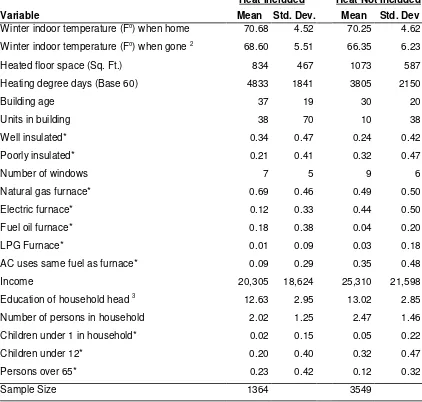
Table 1 compares RECS apartments where heat is included to those in which tenants pay
their own heating bills, weighting the observations to represent all of the apartments in the U.S.
On average, apartments for which heat is included in the rent are kept warmer than those where
tenants pay for heat. The temperature difference is largest when no one is home, indicating that
tenants who pay for heat are more likely to take simple conservation measures such as turning
down the thermostat when leaving home.
Table 1 also suggests reasons why landlords might pay for heating. Apartments where
heat is included in rent are generally found in older, larger buildings, and are more likely to have
a fuel oil heating system. Each of these characteristics is likely to make individual metering of
apartments more difficult and more expensive. Notice also that apartments where landlords pay
11Of course, the causality could run in the other direction. Landlords with individually metered buildings may skimp on energy efficiency investments. In the empirical work that follows we attempt to disentangle these effects.
12The prevalence of heat-included rental contracts varies by region, and by building size and age (tables available from the authors). Older apartments in large buildings in the Midwest and Northeast have the largest fraction of apartments with heat included. However, apartments with heat included exist in all regions and in all age and size classifications.
the same fuel as the heating system, attributes that make the cost to landlords of providing free
heating lower and that are consistent with pre-paid heat as a signal of energy efficiency.11 12
To estimate excess energy use by these tenants, we begin by restricting the sample to
apartments and rental houses that use space heating during the winter and receive no government
aid for heating costs. We only include apartments that use natural gas, fuel oil, electricity, or
liquefied propane gas (LPG) for heating. These comprise 97 percent of the apartments, and
prices for other fuels are not in the RECS.
We assume that tenants choose the interior temperature,T, in order to maximize utility,
given prices, income, and individual preferences. Tis then a function of the marginal cost of an
additional degree of interior temperature,C, income,Y, individual characteristics,X, structural
apartment characteristics,S, and weather,W:
(1)
The marginal cost of heating,C, is determined by several factors. If heat is included in rent the
marginal cost is zero. If the tenant pays for heating, the marginal cost of turning up the
thermostat is determined by the price of heating fuel, weather, and structural characteristics of the
apartment. Thus,
13Fuel prices are non-negative, and skewed, and fit the log-normal distribution well. Electricity and natural gas prices fit best. Heating oil prices are skewed slightly towards zero, relative to the log normal distribution.
14Friedman (1987) notes that, all else equal, the marginal cost of raising the temperature of a home in cold weather is likely to be lower than in warm weather due to the physics of heat loss and possible returns to scale in heating, implying that interior temperatures will be higher in colder climates. This is the indirect effect thatWhas throughCin equation(2). However, whereI=1 if heat is included in rent and zero otherwise, andPis the price of heating fuel. We
estimate a reduced-form version of equation(2):
(3)
The coefficients$and(2reveal the change in temperature in heat-included apartments relative to
metered apartments, controlling for tenant and apartment characteristics.
The price of heating fuel is included in a normalized form. Prices in the RECS are
reported per BTU of energy input, not heating output. Consequently, the price of heat to
consumers is determined by the efficiency of the energy systems used. One BTU of electricity
costs more than one BTU of natural gas, but because electric heating systems are more efficient
(less heat goes up the furnace chimney), the difference in heating costs is less than would be
indicated by the difference in fuel costs. To make prices comparable across fuels, we normalize
each set of fuel prices using a log-normal distribution.13 The remaining variation in fuel prices is
due to differences across regions, over time, and within regions across different energy suppliers.
In the analyses below, we use the normalized fuel price and dummy variables for fuel type to
separate fuel-related and system-related heating cost differences.
We use heating-degree-days (HDD) to control for weather, which could have positive or
Dewees and Wilson (1990) point out that exterior temperatures also directly influence thermostat settings through humidity and air circulation, and the overall effect of outside temperature on thermostat setting is therefore ambiguous.
and indirect effects that make signing the reduced-form coefficients in(5difficult. The variables
included inS, heated floor space, the number of windows, insulation, and building age, all make
the marginal cost of heating more expensive and thus might be expected to lower inside
temperatures. However, since these characteristics also make apartments more drafty and less
comfortable at any given temperature, they may lead to warmer thermostat settings. The tenant
characteristics included inXare education of the head of household, household size, and
indicators for the presence of household members under 5 or over 65 years old.
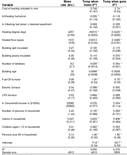
As a benchmark, Table 2 presents ordinary least squares estimates of equation(3), making no adjustment for selection by landlords or tenants into heat-included rental contracts.
The first column presents the means and standard deviations of regressors. The second column
estimates equation(3)where the dependent variable,T, is the winter indoor temperature when someone is home. The third column uses the temperature when nobody is home. In both cases,
the coefficient on the heat-included dummy variable is positive and statistically significant.
Also, as one might expect, the effect is larger in the case when no one is home.
Table 2 includes as regressors normalized heating fuel prices, both alone and interacted
with the metered dummy. We expect, of course, that fuel prices will have a larger effect for
tenants who pay for heating, meaning the interaction term should be negative. While this is true
for both columns, the estimated coefficients (-0.069 and -0.209) are small and statistically
15This type of model is described by Heckman (1976).
16The RECS does not identify landlords, or even buildings, so there is no way to separate landlord and tenant characteristics. Hence, all observations are subscriptedi, and equation(4)
combines the decisions of both landlords and tenants.
The coefficients on the heat-included indicators consistently estimate the true effect of
heat-included rental contracts only if selection into heat-included apartments is exogenous.
However, selection into heat-included and metered apartments is unlikely to be independent of
the heat demand by tenants or the heat-using characteristics of apartments. Two processes
determine this selection. First, the landlord must decide to include heat expenses in the rent of
the apartment. Landlords will be more likely to do so if the metering costs would be relatively
high, and the expected energy costs low. Second, tenants must choose to reside in the apartment,
and they are more likely to do so if they have strong preferences for heating, or are risk averse or
liquidity constrained.
Since we only observe the confluence of these two processes, we cannot separately
identify them. Thus the selection equation is necessarily a reduced form of two separate random
utility models:15
(4)
whereI*is a composite of the relative expenses of the landlord and the relative utility of the
tenants under the two regimes. IfIi*>0 then landlordichooses to include heat in the rent, and
tenantichooses to live there.16
17See, for example, Maddala (1983) Ch. 9.
Once selection by landlords and tenants has been estimated using a probit version of
equation(4), we then model winter indoor temperatures using
(5)
whereTiI is the winter indoor temperature in apartments whose rent includes heat,T i
N is the
winter indoor temperature in apartments whose rent does not include heat, and8i
I=N(0Z i )/(1-M(0Zi)) and8i
N= -N(0Z
i)/M(0Zi) are the selection correction terms.
17 The selection probit
(4)
uses the entire sample, the top heating equation in(5)uses only the observations for which heat is included in rent (I=1), and the bottom heating equation in(5)uses only the observations where heat is not included (I=0). The increase in temperature resulting from heat being included in rent
isTiI-TiNusing predicted values ofTiIandTiNfrom(5).
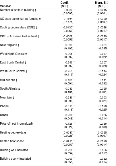
Table 3 gives the coefficients from the first-stage probit, equation(4). We use several instruments for the heat-included variable, all of which should be exogenous to indoor
temperature, and which are excluded from the temperature equations in(5). First, we use the number of units in the apartment building, as larger buildings may have economies of scale from
master-metering. Second, if the apartment has an air conditioner that uses the same fuel as the
heating system, providing free heating will also mean providing free air conditioning, raising the
landlord's cost of including utilities in the rent. And, if the heating fuel also powers an air
conditioning unit, the amount of warm weather in the area will increase the value tenants place
on free utilities and the cost to landlords of providing free utilities, so cooling-degree-days
18We have performed several sensitivity tests of these exclusion restrictions. First, we dropped each of the three excluded variables, instead including them in the second stage: number of units, the air conditioning variables, and the regional dummies. Second, we added building age to the exclusion restrictions by dropping it from the second stage. The key results that follow in Table 4 are robust to these changes. However, tests for joint significance of the exclusion restrictions included in the final stage in each of the sensitivities showed that the null hypothesis that the coefficients on the exclusion restrictions were zero could be rejected in all cases except for the test with the air conditioning variables.
powers both heat and air conditioning. Finally, regional dummies capture potential differences in
regional housing markets that make inclusion of utilities more or less common. These variables
are unlikely to affect thermostat settings, aside from regional differences due to temperature and
fuel prices, both of which are already controlled for in the final stage.
Generally, evidence for both landlord and tenant-side explanations can be seen in Table 3.
On the landlord side, variables associated with higher metering costs, such as building age and
heating costs, are positively associated with heat being included in rent. On the other hand,
heating degree days has a positive coefficient, supporting the signaling-cost landlord-side story.
On the tenant side, poorer tenants and tenants over 65 are more likely to opt for heat included
apartments. Of the variables included in this selection equation but excluded from second stage,
the regional indicators, building size, and cooling degree days are statistically significant.
Although the dummy for air conditioning using the same fuel as heat has the expected large
negative coefficient, it is statistically insignificant.18
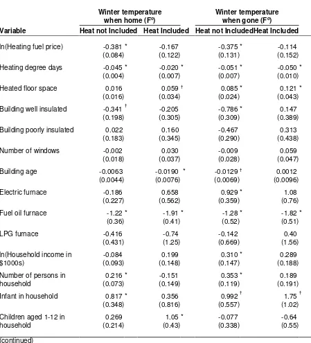
Table 4 shows the results for the second stage regressions. Consistent with our intuition,
fuel price has a larger effect on demand for heating when heat is not included in monthly rents.
both when tenants are home and when they are gone. For heat-included apartments, price has a
smaller and statistically insignificant relationship to temperature.
To calculate the temperature difference between heat-included and metered apartments,
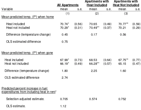
adjusting for selection, in Table 5 we compare the predicted values from Tables 2 and 4. The top
panel displays the difference between predicted temperature settings when somebody is home.
Column (2) calculates this difference using only heat-included apartments, making out-of-sample
predictions for what the temperature settings would be in those apartments if they were
individually metered. Column (3) uses only metered apartments, making out-of-sample
predictions for temperature settings in those apartments if heat were included. And column (1)
calculates this difference for all apartments, making out-of-sample predictions for part of the
data. The difference in each case is less than 1 degree Fahrenheit. The middle panel of the table
shows that same difference when nobody is home, about 2 Fo. The estimated effects are each
smaller in magnitude than the OLS estimates from Table 2 (0.74 Foand 2.82 Fo, respectively),
suggesting that tenants who prefer warmer temperatures self-select into heat-included
apartments.
These results show that tenants who rent apartments with utilities included behave
differently than they would if they paid heating costs separately from rent: they use more heating
and turn back thermostats less when away from home. However, in order to understand the
importance of this effect, we need to translate these temperature settings into fuel use. We can
approximate this translation in two independent ways.
First, to estimate the additional fuel use that results from tenants' reduced conservation
19Because the metered apartments are less well insulated, this procedure overstates the fuel cost per degree of temperature for heat-included apartments. Detailed results are available separately from the authors.
20Note that tenants in heat-included apartments may opt to crank up the heat and open the windows. In that case, our estimate of the additional fuel costs will be an underestimate. In the end, we are going to show that the hedonic rent differences between heat-included and metered apartments is smaller than even these underestimated fuel cost differences.
21CREST web site (http://solstice.crest.org).
22U.S. Department of Energy, Energy Efficiency and Renewable Energy Network, (www.eren.doe.gov/erec/factsheets/thermo.html).
fuel consumption. We regressed the log heating fuel expenditures on log temperature when
home, log temperature when gone, and apartment characteristics, using only the RECS
observations where heat isnotincluded in rent.19 Unsurprisingly, higher temperature settings
correspond to higher fuel use. We then used the coefficients to predict fuel expenditures for each
apartment, both for the case when the landlord pays for heating and the out-of-sample cases
when the tenant pays. The bottom panel of Table 5 presents estimates of the change in fuel
expenditures due to the inclusion of heat in rental contracts. In general the change is small -- less
than one percent.20
As an alternative, we can use published engineering estimates of energy cost savings from
lower temperature settings. According to the Center for Renewable Energy and Sustainable
Technology (CREST), home heating costs fall by 2 percent for every degree the temperature is
lowered.21 Additionally, the U.S. Department of Energy claims that for each degree thermostats
23The average temperature of heat-included apartments is 70.7 Fahrenheit. We estimate that such apartments are 0.46 degrees warmer when the tenants are home, and 1.87 degrees warmer when tenants are gone. Using the CREST estimate for the savings, and assuming tenants are gone for 8 hours each day, this translates to a 2.8 percent higher energy cost in apartments where heat is included in rent.
24SMSA is the only geographic identifier available in the public AHS data.
estimate that energy costs are 1.7 percent higher in heat-included apartments than they would be
if these same apartments, with the same tenants, were individually metered.23
As we suggested in the introduction, tenants in heat-included apartments value this extra
heat at less than its marginal cost. If the premium for heat-included apartments is less than the
utility costs, that will support landlord-side explanations for these inefficient rental contracts, and
if the rent premium makes up for the increased utility costs, that would support tenant-side
explanations. To try to distinguish between the landlord-side and tenant-side explanations, we
next examine data on the rent differences between utility-included and metered apartments.
Rent differences for utility-included apartments
Because the RECS contains no information about rents, we instead turn to the American
Housing Survey (AHS), a biennial survey conducted by the Bureau of the Census for the
Department of Housing and Urban Development. We use the 1985 through 1997 national core
samples, limited to apartments not subject to rent control and for which metropolitan area is
identified.24 The sample contains 31,293 rental units from 148 metropolitan areas.
The AHS describes the fuels used in each apartment, identifies who pays the various
utility costs, and reports the monthly rent. Among the variables in the AHS are several related to
25As in the RECS data, AHS apartments that are older, in larger buildings, and in the Northeast and Midwest are more likely to have heat included in the rent (details available separately). However, building size, age, and region do not explain all of the variation in metering arrangements. The RECS and the AHS differ substantially, as can be seen by
comparing tables 2 and 6. The principal difference is that the AHS contains only apartments in metropolitan areas (SMSAs).
For apartments where tenants pay for utilities, the data contain the average monthly costs of
water, gas, and electricity.
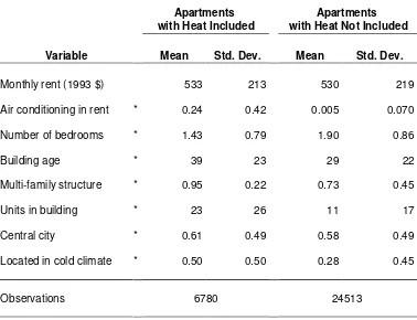
Table 6 compares AHS apartments where tenants pay for heat to those where heat is
included in the rent. The average rent is not statistically significantly larger in apartments where
heat is included. However, these heat-included apartments are smaller and older, and more likely
to be in larger, multi-family buildings.25
We use the AHS to compare the rent paid by tenants in heat-included apartments to the
rent paid by other tenants. This approach is an application of the hedonic price model outlined
by Rosen (1974). We estimate
(6)
whereRenti is monthly apartment rent,Iiis a dummy for inclusion of heat in rent,Xiis a vector
of apartment characteristics related to the cost of heating (and thus the value of free heat), andZi
is a vector of other apartment characteristics, including dummy variables for each of 148
metropolitan areas.
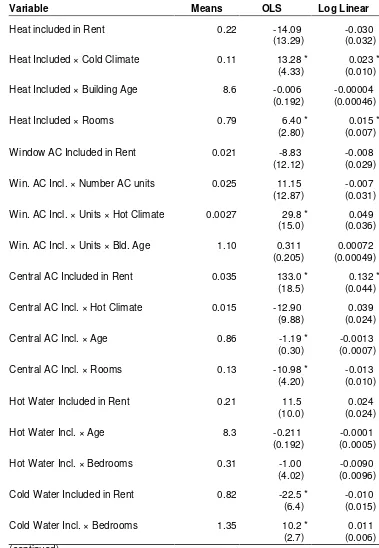
Table 7 presents two different specifications of equation(6): an OLS regression with the dollar value of rent as the dependent variable, and a log-linear specification. Each contains
26Results available separately from the authors.
And, because we expect the rent premium for included utilities to be larger depending on their
expected usage, we include interaction terms between these dummy variables and apartment
characteristics related to the utility usage: climate dummies, building age, and apartment size. At
the bottom of Table 7 we calculate the average premium for heat-included rents. As expected,
rents are higher when utilities are paid by the landlord. The linear and log-linear estimates are
very similar. The results from Table 7, calculated at the average values in the data, predict that
including heat in utilities raises rent by about 4 percent, or $17 per month.
Because hedonic models are typically estimated for individual cities, rather than a
national sample, we have also estimated models similar to Table 7 separately for the 14
metropolitan areas most heavily represented in the AHS.26 Many of the coefficients are
imprecisely estimated, in part because of the smaller sample sizes, but all of the statistically
significant coefficients are large and positive, and follow a sensible pattern given cities' climates.
(Boston rents are significantly higher when heat is included, while Washington, DC rents are
higher when AC is included).
To determine if these rent premiums fully offset the extra energy used by heat-included
apartments, the premiums for free utilities need to be compared to the utility bills in apartments
where tenants pay the cost directly. Unfortunately, unlike the RECS, the AHS does not provide
separate measures of different utility uses such as heating and air conditioning. Instead, the AHS
provides thetotalutility bills for all purposes. We therefore compare the estimated increase in
where the tenants payallutility bills. Table 8 presents these comparisons by apartment size and
region.
These comparisons reveal, to a rough approximation, who bears the inefficiency cost of
heat-inclusive rental contracts, and why they exist. If landlord-side costs explain their existence,
then the implicit price of free utilities will be less than the average costs of utilities in metered
apartments, inflated to account for the extra utility use by tenants facing zero marginal costs. If
tenant preferences explain the persistence of heat-included rental contracts, then the implicit
price of free utilities will fully compensate landlords for the extra costs they incur. The
AHS-based analysis in Table 7 provides the implicit price for including utilities, and the RECS-AHS-based
analysis in Table 4 provides the increased energy use when heat is included in rent.
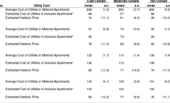
The top line of Table 8 contains the average utility bill, for all utilities, for those
apartments where the tenants pay for utilities, calculated from the AHS. The second line presents
that average utility bill inflated by 2 percent, a rough estimate of the increase in usage from the
RECS survey, and the engineering estimates in footnote 23. The third line presents the hedonic
price of having all utilities included in rent, calculated from Table 7.
With the exception of one-bedroom apartments in cold climates, the increase in rent is
never large enough to offset the costs of utilities, even before the 2 percent increase, and for 3
and 4-bedroom apartments the differences are statistically significant. This suggests that
landlord-side explanations account for at least part of the inclusion of heat in rent, since landlords
do not appear to recover the full cost of doing so. Why would landlords include utilities in their
rental contracts despite consumers' unwillingness to pay increased rent sufficient to offset the
or because their energy efficiency investments cannot otherwise be passed through to uncertain
renters.
Conclusion
The intuition outlined in Figure 1 suggests that in a perfectly competitive market,
landlords will never include heating or cooling costs in rents. Yet in practice they often do.
Either landlords or tenants value utility-included apartments more than the extra energy costs. In
the former case, we should expect the rent differential to less than fully compensate landlords for
their energy expenditures. In the latter case, landlords will be fully compensated.
We find that tenants in heat-included apartments do use more energy,ceteris paribus, but
that the additional utility costs are not large. If tenants are risk averse, do not want volatile utility
bills, or simply prefer not facing the marginal cost of energy, they may be willing to pay this
small additional cost. However, we also find that the implicit cost of free utilities, paid as higher
rents, is less than the utility costs in metered apartments. So while we cannot rule out the
presence of tenant demand for heat-included arrangements, some of the explanation for the
persistence of heat-included rental contracts must come from landlord-side explanations:
metering costs, economies of scale, or signaling costs.
However, Figure 1 does not describe the entire set of inefficiencies confronting
residential apartments' energy use. A second inefficiency occurs if landlordsdo notinclude the
cost of utilities in monthly rents -- such landlords have little incentive to invest in energy
efficient construction, appliances, or insulation. Indeed, we have shown that heat-included
the causality flows. Landlords of heat-included apartments may provide more energy efficiency
to minimize costs, or landlords of energy-efficient apartments may lease them with utilities
included to signal their efficiency. Nevertheless, it does appear that the inefficient energy use by
tenants in utility-included apartments is at least partly offset by the increased energy efficiency of
such apartments.
Policies that encourage the inclusion of energy costs in base rents would be appropriate if
having landlords responsible for utilities led to greaterefficiency, via investments in energy
efficient construction. However some policies, such as PURPA and the federal buildings
guidelines, explicitly encourage individual metering. This would be appropriate if having
landlords responsible for utilities led to greaterinefficiency, in the form of wasteful use by
tenants. Our findings indicate that landlord-side explanations underlie utility-included rental
contracts, but this is not quite enough information to discern which set of federal policies is more
appropriate.
To assess fully the welfare and policy implications of landlord costs, we need to know
whichof the landlord-side explanations is most important. If landlords use utility-included
apartments to signal energy efficiency, that may represent a second-best market solution to an
information asymmetry. Prohibited from including utilities, landlords might be unable to
capitalize on energy efficiency investments, and might not make those investments.
Distinguishing among the various landlord-side explanations for heat-included rent, however, is
References
Akerlof, George A. 1970. The Market for 'Lemons': Quality Uncertainty and the Market Mechanism. Quarterly Journal of Economics84(3), 488-500.
Asabere, P.K. and C. McGowan. 1987. Some Factors Explaining Variations in Rents of Downtown Apartments for 49 Cities of the World. Urban Studies24: 279-84.
Baker P., R. Blundell, and J. Micklewright. 1989. Modelling Household Energy Expenditures Using Micro-Data. Economic Journal99: 720-38.
Branch, R.E. 1993. Short Run Income Elasticity of Demand for Residential Electricity Using Consumer Expenditure Survey Data. Energy Journal14: 111-21.
Dewees, D.N. and T.A. Wilson. 1990. Cold Houses and Warm Climates Revisited: On Keeping Warm in Chicago, or Paradox Lost. Journal of Political Economy98: 656-63.
Dubin, J.A., A.K. Miedema, and R.V. Chandran. 1986. Price Effects of Energy-Efficient
Technologies: A Study of Residential Demand for Heating and Cooling. Rand Journal of Economics17: 310-25.
Dubin, J.A. and D. McFadden. 1984. An Econometric Analysis of Residential Electric Appliance Holdings and Consumption. Econometrica 345-62.
Friedman, D. 1987. Cold Houses in Warm Climates and Vice Versa: A Paradox of Rational Heating. Journal of Political Economy95: 1089-97.
Gillingham, R. and R.P. Hagemann. 1984. Household Demand for Fuel Oil.Applied Economics 16: 475-82.
Hassett K., and G. Metcalf. 1995. Energy Tax Credits and Residential Conservation Investment: Evidence from Panel Data.Journal of Public Economics57(2): 201-17.
Hassett K., and G. Metcalf. 1999. Measuring the Energy Savings From Home Improvement Investments: Evidence from Monthly Billing Data,"Review of Economics and Statistics 81(3): 516-528.
Hausman, J.A. 1979. Individual Discount Rates and the Purchase and Utilization of Energy Using Durables. Bell Journal of Economics10: 33-54.
Jaffe, A.B. and R. Stavins. 1994. The Energy Efficiency Gap: What Does It Mean?Energy Policy22: 804-810.
Jaffe, A.B. and R. Stavins. 1994. The Energy Paradox and the Diffusion of Conservation Technology.Resource and Energy Economics16: 91-122.
Jaffe, A.B. and R. Stavins. 1994. Energy-Efficiency Investments and Public Policy.The Energy Journal15(2): 43-65.
Maddala, G.S. 1983. Limited Dependent and Qualitative Variables in Econometrics. Cambridge University Press, New York.
Munley, V.G., Taylor, L.W. and Formby, J.P. 1990. Electricity Demand in Multi-family, Renter-Occupied Residences. Southern Economic Journal57(1): 178-94.
Table 1
Comparison of RECS Apartments With and Without Heat Included in Rent1 (Means Weighted to Represent All U.S. Apartments)
Heat Included Heat Not Included
Variable Mean Std. Dev. Mean Std. Dev
Winter indoor temperature (Fo) when home 70.68 4.52 70.25 4.62
Winter indoor temperature (Fo) when gone2 68.60 5.51 66.35 6.23
Heated floor space (Sq. Ft.) 834 467 1073 587
Heating degree days (Base 60) 4833 1841 3805 2150
Building age 37 19 30 20
Units in building 38 70 10 38
Well insulated* 0.34 0.47 0.24 0.42
Poorly insulated* 0.21 0.41 0.32 0.47
Number of windows 7 5 9 6
Natural gas furnace* 0.69 0.46 0.49 0.50
Electric furnace* 0.12 0.33 0.44 0.50
Fuel oil furnace* 0.18 0.38 0.04 0.20
LPG Furnace* 0.01 0.09 0.03 0.18
AC uses same fuel as furnace* 0.09 0.29 0.35 0.48
Income 20,305 18,624 25,310 21,598
Education of household head3 12.63 2.95 13.02 2.85
Number of persons in household 2.02 1.25 2.47 1.46 Children under 1 in household* 0.02 0.15 0.05 0.22
Children under 12* 0.20 0.40 0.32 0.47
Persons over 65* 0.23 0.42 0.12 0.32
Sample Size 1364 3549
Source: U.S. Energy Information Administration, 1987, 1990, 1993, 1997 Residential Energy Consumption Survey.
1Differences between the heat-included apartments and the metered apartments are all statistically
significant at 5 percent.
2Temperature when gone only observed for 1213 heat-included apartments and 2716 metered
apartments.
21987-1993 only. Education was dropped from the RECS after 1993, so the analyses that follow do not
control for education. We have estimated all of the models using only data for 1993 and earlier, and included education, with virtually identical results.
Table 2
Cost of heating included in rent 0.749 * 2.74 *
(0.167) (0.24)
ln(Heating fuel price) -0.226† -0.119
(0.116) (0.160)
ln (Heating fuel price) x metered apartment -0.069 -0.209 (0.142) (0.201)
Heating degree days 4257 -.00315 * -0.0425 *
(2155) (0.0033) (0.0050)
Heated floor space 1010 -0.0013 0.0469 *
(576) (0.0134) (0.0191)
Building well insulated 0.27 -0.155 -0.173
(0.44) (0.162) (0.238)
Building poorly insulated 0.30 -0.110 -0.570 *
(0.46) (0.156) (0.234)
Number of windows 8.2 -0.028† -0.054 *
(5.7) (0.0014) (0.021)
Building age 32 -0.0068† -0.0028
(20) (0.0038) (0.0055)
Fuel Oil furnace 0.09 -1.30 * -0.70 *
(0.29) (0.24) (0.33)
Electric furnace 0.34 -0.399 * -0.000
(0.47) (0.162) (0.248)
LPG furnace 0.03 -0.884 * -0.699
(0.17) (0.400) (0.590)
ln (household income in $1000s) 23085 -0.076 0.204†
(20920) (0.077) (0.114)
Number of persons in household 2.43 0.135 * 0.293 *
(1.44) (0.066) (0.101)
Infants in household 0.047 0.623† 0.908†
(0.211) (0.321) (0.484)
Children aged 1-12 in household 0.31 0.362† -0.303
(0.46) (0.192) (0.287)
Persons over 65 in household 0.14 1.46 * 1.92 *
(0.35) (0.20) (0.29)
Intercept 71.8 * 66.7 *
(0.34) (0.53)
R2 0.055 0.075
Sample size 4913 4913 3929
Standard errors in parentheses.
Table 3 Selection Model First Stage Probit
Dependent Variable = Heat Included in Rent
Variable
Coeff. (S.E.)
Marg. Eff. (S.E.)
Number of units in building ‡ 0.0052 * 0.0015 (0.0005) (0.0001) AC uses same fuel as furnace ‡ -0.1164 -0.0330
(0.1471) (0.0407) Cooling degree days (CDD) ‡ 0.0130* 0.0038
(0.0060) (0.0017) CDD × AC same fuel as heat ‡ -0.0068 -0.0020
(0.0059) (0.0017)
New England ‡ 0.269 * 0.084
(0.103) (0.035)
West North Central ‡ -0.296 * -0.077
(0.097) (0.022)
East South Central ‡ -0.296 * -0.067
(0.097) (0.028)
West South Central ‡ -0.253 * -0.114
(0.119) (0.024)
Mid-Atlantic ‡ 0.435 * 0.141
(0.091) (0.032)
South Atlantic ‡ 0.083 0.025
(0.101) (0.031)
Mountain ‡ -0.236 * -0.063
(0.099) (0.024)
Pacific ‡ -0.513 * -0.128
(0.118) (0.025)
Urban 0.230 * 0.066
(0.048) (0.014)
Price of heat (normalized) -0.126 * -0.036
(0.029) (0.009)
Heating degree days 0.0087 * 0.0025
(0.0025) (0.0007)
Heated floor space -0.0415 * -0.0120
(0.0050) (0.0014)
Building well insulated 0.220 * 0.066
(0.054) (0.017)
Building poorly insulated -0.299 * -0.082
(Table 3, continued)
Number of windows -0.053 * -0.015
(0.005) (0.002)
Electric furnace -0.928 * -0.235
(0.096) (0.021)
Fuel oil furnace 0.375 * 0.121
(0.085) (0.030)
LPG furnace -0.443 * -0.106
(0.158) (0.030)
Building age 0.0049 * 0.0014
(0.0013) (0.0004) Household income ($1000s) -0.00609 * -0.00177
(0.00129) (0.00037) Number of persons in household -0.0145 -0.0042
(0.0240) (0.0070)
Infant in household -0.257 * -0.067
(0.122) (0.028)
Child aged 1-12 in house -0.082 -0.023
(0.069) (0.019)
Person over 65 in household 0.219 * 0.067
(0.064) (0.021)
Intercept -0.181
(0.215)
Number of observations 4913
Standard errors are reported in parentheses. * Statistically significant at 5 percent.
Table 4
Variable Heat not Included Heat Included Heat not IncludedHeat Included
ln(Heating fuel price) -0.381 * -0.167 -0.375 * -0.114
(0.084) (0.122) (0.131) (0.152)
Heating degree days -0.045 * -0.020 * -0.051 * -0.050 *
(0.004) (0.007) (0.007) (0.010)
Heated floor space 0.016 0.059† 0.085 * 0.121 *
(0.016) (0.034) (0.024) (0.043)
Building well insulated -0.341† -0.205 -0.786 * 0.147
(0.198) (0.305) (0.309) (0.389)
Building poorly insulated 0.022 0.160 -0.467 0.313
(0.183) (0.345) (0.290) (0.438)
Number of windows -0.002 0.030 -0.009 0.059
(0.018) (0.037) (0.028) (0.047)
Building age -0.0063 -0.0190 * -0.0129† 0.0012
(0.0044) (0.0076) (0.0069) (0.0096)
Electric furnace -0.186 0.658 0.929 * 1.08
(0.227) (0.562) (0.359) (0.76)
Fuel oil furnace -1.22 * -1.91 * -1.28 * -1.82 *
(0.36) (0.41) (0.52) (0.51)
LPG furnace -0.416 -0.74 -0.142 0.40
(0.431) (1.25) (0.669) (1.56)
ln(Household income in $1000s)
-0.084 0.199 0.310 * 0.289
(0.093) (0.148) (0.147) (0.188)
Number of persons in household
0.216 * -0.151 0.353 * 0.189
(0.073) (0.149) (0.119) (0.191)
Infant in household 0.817 * 0.356 0.992† 1.75†
(Table 4 continued) Persons over 65 in household
1.27 * 1.06 * 2.04 * 0.96 *
(0.25) (0.35) (0.40) (0.44)
Selectivity regressor (8) -1.79 * -1.11 * -2.26 * -2.80 *
(0.45) (0.52) (0.68) (0.68)
Intercept 70.9 * 72.2 * 65.1 * 70.7 *
(0.49) (0.70) (0.79) (0.91)
R2 0.068 0.048 0.059 0.050
Observations 3549 1364 2716 1213
Standard errors are reported in parentheses.
Table 5
Average Predicted Winter Indoor Temperature (Fo)
Variable
mean s.e. mean s.e. mean s.e.
(1) (2) (3)
Mean predicted temp. (Fo) when home
Heat included 70.74* (0.56) 70.65 (0.49) 70.77** (0.59) Heat not included 70.29* (0.31) 70.49** (0.37) 70.21 (0.29) Difference (temperature change) 0.45 0.17 0.56
OLS estimated difference 0.75
Mean predicted temp. (Fo) when gone
Heat included 67.99* (0.73) 68.53 (0.64) 67.75** (0.77) Heat not included 66.19* (0.49) 66.28** (0.57) 65.15 (0.47) Difference (temperature change) 1.80 2.25 1.60
OLS estimated difference 2.74
Predicted percent increase in fuel expenditures from including heat in rent1
Selection adjusted estimate. 0.705 0.574 0.752
OLS estimate. 1.12
1
Applies predicted fuel expenditures from a regression of log(annual fuel expenditures) on winter temperature when home and away, and apartment characteristics. (Available separately from the authors.)
* Partly out-of-sample prediction. ** Out-of-sample prediction.
Note: For each observation in the data set, we obtained a predicted value for each case (heat included or not), using the sampling weights in the RECS. In the OLS
Table 6
Selected Means for AHS Apartments With and Without Heat-Included in Rent Means Weighted to Represent All U.S. Apartments
1985, 1987, 1989, 1991, and 1993
Apartments with Heat Included
Apartments with Heat Not Included
Variable Mean Std. Dev. Mean Std. Dev.
Monthly rent (1993 $) 533 213 530 219
Air conditioning in rent * 0.24 0.42 0.005 0.070
Number of bedrooms * 1.43 0.79 1.90 0.86
Building age * 39 23 29 22
Multi-family structure * 0.95 0.22 0.73 0.45
Units in building * 23 26 11 17
Central city * 0.61 0.49 0.58 0.49
Located in cold climate * 0.50 0.50 0.28 0.45
Observations 6780 24513
Table 7 Hedonic Rent Model
Dependent Variable = Monthly Rent
Variable Means OLS Log Linear
Heat included in Rent 0.22 -14.09 -0.030 (13.29) (0.032) Heat Included × Cold Climate 0.11 13.28 * 0.023 *
(4.33) (0.010) Heat Included × Building Age 8.6 -0.006 -0.00004
(0.192) (0.00046) Heat Included × Rooms 0.79 6.40 * 0.015 *
(2.80) (0.007) Window AC Included in Rent 0.021 -8.83 -0.008
(12.12) (0.029) Win. AC Incl. × Number AC units 0.025 11.15 -0.007
(12.87) (0.031) Win. AC Incl. × Units × Hot Climate 0.0027 29.8 * 0.049
(15.0) (0.036) Win. AC Incl. × Units × Bld. Age 1.10 0.311 0.00072
(0.205) (0.00049) Central AC Included in Rent 0.035 133.0 * 0.132 *
(18.5) (0.044) Central AC Incl. × Hot Climate 0.015 -12.90 0.039
(9.88) (0.024) Central AC Incl. × Age 0.86 -1.19 * -0.0013
(0.30) (0.0007) Central AC Incl. × Rooms 0.13 -10.98 * -0.013
(4.20) (0.010) Hot Water Included in Rent 0.21 11.5 0.024
(10.0) (0.024) Hot Water Incl. × Age 8.3 -0.211 -0.0001
(0.192) (0.0005) Hot Water Incl. × Bedrooms 0.31 -1.00 -0.0090
(4.02) (0.0096) Cold Water Included in Rent 0.82 -22.5 * -0.010
(6.4) (0.015) Cold Water Incl. × Bedrooms 1.35 10.2 * 0.011
(Table 7 continued)
Bedrooms 1.80 35.7 * 0.078 *
(2.4) (0.006)
Bathrooms 1.24 68.7 * 0.104 *
(2.4) (0.006)
Other Rooms 1.12 10.8 * 0.023 *
(1.3) (0.003) Floor of Apartment Building 0.92 4.28 * 0.006 *
(0.83) (0.002)
Single Family Home 0.14 44.4 * 0.050 *
(3.5) (0.008) Single Family Home (Attached) 0.061 13.1 * 0.00008
(3.8) (0.00902)
Building Age 32.4 -2.63 * -0.0048 *
(0.17) (0.0004) Building Age Squared 1580 0.023 * 0.000035 *
(0.002) (0.000005)
Near a Park 0.16 -4.18 -0.012 *
(2.38) (0.006) Near a Body of Water 0.040 28.8 * 0.052 *
(4.5) (0.011) Near Abandoned Buildings 0.048 -49.0 * -0.121 *
(4.1) (0.010) Bars on Nearby Windows 0.15 -22.0 * -0.046 *
(2.7) (0.006) Exterior in Poor Condition 0.17 -4.19 -0.0112 *
(2.4) (0.0057) Walls or Floor in Poor Condition 0.11 -18.3 * -0.039 *
(2.8) (0.007)
Water Leaks In 0.12 -0.33 -0.0022
(2.58) (0.0062) Number of Units in Building 13.5 0.451 * 0.00088
(0.063) (0.00015) Number of Stories in Building 2.66 7.19 * 0.013 *
(1.05) (0.003)
Washer/Dryer 0.29 26.5 * 0.055 *
(2.3) (0.005)
Dishwasher 0.43 62.7 * 0.123 *
(Table 7 continued)
Free Garage Parking 0.33 48.4 * 0.110 *
(3.1) (0.007) Free Off Street Parking 0.47 16.3 * 0.047 *
(2.8) (0.007)
Porch or Patio 0.61 3.12 * 0.0079
(1.94) (0.0046)
Fireplace 0.14 57.6 * 0.092 *
(2.8) (0.007)
Central AC 0.38 40.9 * 0.113 *
(3.1) (0.008)
Window AC 0.30 8.1 * 0.021 *
(2.4) (0.006)
Central City 0.56 -12.6 * -0.034 *
(2.1) (0.005) Dummies for years (7) and
metropolitan areas (148).
not reported
--Predicted rent premium for heat included, based on averages for climate, age, and rooms.
+17.08 +0.041
R2 0.551 0.448
Observations 31,293 31,293
Heteroskedasticity-consistent standard errors in parentheses. * Statistically significant at 5 percent.
Table 8
Average Monthly Cost of Utilities in Metered Apartments vs. Implicit Hedonic Price of Free Utilities**
Cold Climate Moderate Climate Hot Climate
Apartment type Utility Cost mean s.e. mean s.e. mean s.e.
1 Bedroom Apartments
Average Cost of Utilities in Metered Apartments $68 (1.0) $56 (0.7) $65 (0.8)
Estimated Cost of Utilities in Inclusive Apartments* 69 57 66
Estimated Hedonic Price 74 (11.1) 61 (9.3) 59 (10.4)
2 Bedroom Apartments
Average Cost of Utilities in Metered Apartments 91 (0.9) 74 (0.6) 92 (1.0)
Estimated Cost of Utilities in Inclusive Apartments* 93 75 94
Estimated Hedonic Price 79 (11.3) 66 (9.6) 65 (10.8)
3 Bedroom Apartments
Average Cost of Utilities in Metered Apartments 123 (1.7) 110 (1.4) 126 (1.9)
Estimated Cost of Utilities in Inclusive Apartments* 126 112 128
Estimated Hedonic Price 85 (11.6) 71 (10.2) 70 (11.3)
4+ Bedroom Apartments
Average Cost of Utilities in Metered Apartments 140 (4.1) 139 (3.8) 151 (6.2)
Estimated Cost of Utilities in Inclusive Apartments* 143 142 154
Estimated Hedonic Price 90 (13.2) 77 (9.9) 76 (11.1)
* Assuming a 2 percent increase in consumption, as estimated for heating using the RECS, and footnote 23.
Unpublished Appendix Table 1 (Available from the authors)
Percentage of Apartments with Heat Included in the Rent
By Age, Census Region, and Building Size1
Built Before 1950 Built 1950-1979 Built after 1979
Region
Northeast 40.4 89.7 98.7 52.0 63.8 85.1 7.0 18.0 45.8
Midwest 29.6 72.7 94.4 2 28.7 62.9 86.9 8.1 40.5 58.3
South 14.5 75.0 40.0 2 18.6 27.6 73.5 8.8 3.1 10.7
West 20.1 33.9 12.5 2 15.9 33.2 32.2 7.3 1.8 8.3
Source: Energy Information Administration, 1987, 1990, 1993 and 1997 Residential Energy Consumption Survey.
1Small = 8 or fewer apartments; Medium = 9 - 29 apartments; Large = 30+ apartments.
Unpublished Appendix Table 2 (Available from the authors)
Percentage of Apartments with Heat Included in the Rent
By Age, Census Region, and Building Size1
Built Before 1950 Built 1950-1979 Built after 1979
Region
Northeast 28.9 62.0 73.9 27.6 52.1 72.8 6.4 23.2 53.0
Midwest 16.1 39.6 65.3 18.3 37.4 49.0 4.6 7.7 33.6
South 12.0 42.5 32.6 8.9 15.6 19.4 1.7 2.5 14.9
West 11.4 30.5 53.9 7.5 16.5 22.6 4.9 2.7 17.8
Source: American Housing Survey 1985, 1987, 1989, 1991, 1993, 1995, and 1997.
Unpublished Appendix Table 3 (Available from the authors) Hedonic Rent Models for Individual Cities
City
Anaheim1 -37.13 * 0.577 645 13%
(16.13)
Boston 24.73 0.327 710 39%
(17.55)
Chicago 34.02 * 0.382 1702 33%
(9.17)
Dallas 7.92 0.474 806 17%
(28.15)
Detroit1 22.43 0.548 771 26%
(11.65)
Houston 29.81 0.498 786 16%
(27.74)
Los Angeles -10.83 0.504 2571 10% (11.54)
New York2 -12.96 0.257 1914 62%
(10.40)
Philadelphia 31.76 * 0.477 858 33% (13.05)
Washington, DC
12.96 0.569 635 53%
(19.49)
Minneapolis1 8.76 0.709 489 44%
(10.16)
Milwaukee1 35.84 * 0.526 351 26%
(17.47)
Buffalo1 12.37 0.493 235 27%
(21.95) *Statistically significant at 5 percent.
1 Indicator variable for AC Included in rent excluded because landlord
pays bill for very few apartments.
2 Indicator variable for water included in rent excluded because tenants
Unpublished Appendix Table 4 (Available from the authors)
Fuel Use and Winter Indoor OLS Estimates from
Metered Apartments in RECS Sample
Dependent Variable = ln (Annual expenditure on fuel)
Variable
Coeff. (S.E.)
ln (Temperature when home) 0.549 * (0.203) ln (Temperature when gone) 0.137
(0.129)
Heating degree days 0.019 *
(0.001)
Heated floor space 0.022 *
(0.002)
Building well insulated -0.038
(0.028) Building poorly insulated 0.141 *
(0.026)
Number of windows 0.037 *
(0.002)
Electric furnace -0.0076
(0.0264)
Fuel Oil furnace 0.099 *
(0.046)