Mathematical methods and models1

(1)

Diss. ETH No. 16357

Comparative Investigation of

Mathematical Methods for

Modeling and Optimization of

Common-Rail DI Diesel Engines

A thesis submitted to the

SWISS FEDERAL INSTITUTE OF TECHNOLOGY

ZURICH

for the degree of

DOCTOR OF TECHNICAL SCIENCES

presented by

MARCO WARTH

Dipl. Masch.-Ing. ETH Zürich

born April 10, 1976

Citizen of Ruswil and Gunzwil, LU

Accepted of the recommendation of

Prof. Dr. K. Boulouchos, examiner

Prof. Dr. Ph. Rudolf von Rohr, co-examiner

(2)

(3)

“To walk uncommon paths, one has to know the old ways and seek for the new ones.”

(4)

(5)

A

CKNOWLEDGMENTS

This thesis was written during my work as a research associate with the Aerothermo-chemistry and Combustion Systems Laboratory (LAV) at the Swiss Federal Institute of Technology in Zurich.

Above all, I would to thank Prof. Dr. Konstantinos Boulouchos - who has both promoted my interest in this topic and guided my work - for his interest, his support and for our various motivating discussions. My gratitude also goes to Prof. Dr. Phil-ipp Rudolf von Rohr for his interest in this work and for his time and efforts acting as co-examiner.

I would also like to thank Peter Obrecht for the excellent collaboration during the development and implementation of the phenomenological models.

For providing me with a unique set of experimental engine data, the generosity and support of Dr. Andrea Bertola, Klaus Heim, Dr. German Weisser, and Dr. Georgios Bikas are greatly appreciated.

Last but not least, special thanks go to:

• Pat Kirchen for both the scientific and personal discussions, the expert proofreading of this thesis and for teaching me the canadian way of life, • Daniel Fritsche and Dr. Marc Füri for being comrades in arms and mind

-for the past three years,

• all the colleagues from LAV for the good collaboration,

• “Rusmu & Sorsi förs Verständnis, d’Onderschtötzig ond s’Bänzin im Bluet” • and all those not mentioned here, who are in my mind for contributing, in

any way, to the success of this work.

(6)

(7)

A

BSTRACT

In the following work, a phenomenological/knowledge based model and a “black-box” approach for the simulation and optimization of Common-Rail DI diesel engines are developed and comparatively evaluated. The evaluation, which is carried out for a comprehensive sample of engines and operating conditions, focuses on the ability of both approaches to yield predictive measures of the in-cylinder combustion process, as well as the engine out exhaust emissions.

The phenomenological/knowledge based model expands an existing, simple, yet physically and chemically accurate model by implementing Evolutionary Algorithms to calibrate the model parameters. As is shown through comprehensive investiga-tions using measurements from an automotive, a heavy-duty, and a two-stroke marine diesel engine, the new models are able to determine the qualitative and quan-titative Rates Of Heat Release (ROHR), nitrogen oxide and soot emissions across an entire engine operating map within a matter of seconds. To evaluate the general applicability of the model, a version of the model calibrated to one engine (for exam-ple the heavy-duty engine) is directly applied to another engine (for examexam-ple the marine diesel engine), without recalibrating the model parameters. For such a “blind try” investigation, it is seen that because the phenomenological model considers the appropriate physical and chemical processes, it is capable of providing extrapolative predictions.

In addition to evaluating the model based on a comparison of calculations and mea-surements from applied combustion systems, a detailed investigation of the model itself is carried out. In particular, a sensitivity analysis of the model specific param-eters and statistical analyses are used to evaluate the modeling and optimization per-formance of the model. From such an analysis of the ROHR model, it is shown, among other things, that: (i) the accuracy of the model depends on the calibration algorithm, (ii) there are only negligible differences due to stochastic parameter initial-ization when using Evolutionary Algorithms, and (iii) the chemical and physical effects seen during the implementation of alternative fuels, such as diesel-water emulsions and diesel-butylal blends are correctly represented by the ROHR sub-model. Furthermore, from the detailed analysis of the emission models, a larger sen-sitivity of the model to small parameter changes is seen, as is a general influence of the operating conditions on the model accuracy.

(8)

variables, with the exception of the maximum rate of pressure rise.

As an alternative to the phenomenological/knowledge based model approach, an Artificial Neural Network (ANN) is also investigated as a representative “black-box” approach. From a comparison of these two approaches, based on their abilities to predict ROHR parameters, nitrogen oxide and soot emissions, it is seen, that the ANN is more easily adapted to different engine configurations and provides better agreement with the measured calibration (i.e. training) data. However, when the models are used to predict the ROHR characteristics and exhaust emissions for operating conditions to which they were not trained, the ANN is not able to match the extrapolative ability of the phenomenological/knowledge based model, which provides better agreement with the measured values.

(9)

Z

USAMMENFASSUNG

Gegenstand der vorliegenden Arbeit ist die Herleitung und vergleichende Untersu-chung eines modell-/wissensbasierten und eines “black-box” Ansatzes zur innermo-torischen Simulation und Optimierung der Verbrennung sowie Schadstoffent-stehung in direkt eingespritzten Common-Rail Diesel Motoren. Die hierzu entwik-kelten Ansätze und Modelle werden für eine umfangreiche Palette von unterschied-lichen Motoren und Betriebszustände angewandt.

Der neu entwickelte, modell-/wissensbasierte Ansatz baut auf einfachen, jedoch physikalisch und chemisch korrekten phänomenologischen Modellen auf, welche mittels evolutionärer Algorithmen kalibriert werden. Wie in umfangreichen Untersu-chungen an einem Automobil-, einem Nutzfahrzeug-, und einem Schiffsantrieb erfolgreich gezeigt werden konnte, erlaubt der Ansatz die kennfeldweite, qualitative und quantitative Berechnung von Brennverläufen, Stickoxid- und Russemissionen innerhalb weniger Sekunden. Anhand von sogenannten “blinden Versuchen”, in welchen kalibrierte Modelle eines Motors ohne Anpassung der Parameter auf einen anderen Motor übertragen wurden (z.B. das für den Nutzfahrzeugmotor kalibrierte Brennverlaufsmodell wird zur Berechnung des Schiffsantriebs verwendet), konnte des weiteren gezeigt werden, dass die Verwendung geeigneter physikalisch/che-misch basierter Modelle selbst extrapolative Abschätzungen ermöglicht.

Neben den stark anwendungsorientierten Vergleichen von experimentellen und berechneten Kenngrössen für die jeweiligen Betriebspunkte wurden für alle Modelle auch detaillierte Untersuchungen (z.B. Parameter Sensitivitätsstudien) und statisti-sche Analysen zu speziellen Modellierungs- und Optimierungsaspekten durchge-führt. Die detaillierte Analyse der Brennverlaufsmodellierung ergab dabei unter anderem eine differenzierte Abhängigkeit der Modellqualität von verschiedenen Kalibrierungsalgorithmen, vernachlässigbare Abweichungen aufgrund stochasti-schen Parameterinitialisierung bei evolutionären Algorithmen, sowie die korrekte Abbildung der physikalischen und chemischen Einflüsse unterschiedlicher Kraft-stoffe wie Diesel-Wasser-Emulsionen oder Diesel-Butylal-Gemische. Am Beispiel der Schadstoffmodellierungen konnten ferner stark unterschiedliche Sensitivitäten der Modelle sowohl bei geringen Parameteränderungen, als auch zwischen verschie-denen Betriebspunkten im Allgemeinen, gezeigt werden.

(10)

(11)

T

ABLE

OF

C

ONTENTS

ACKNOWLEDGMENTS_...V

ABSTRACT ... VII

ZUSAMMENFASSUNG ... IX

TABLEOF CONTENTS ... XI

LISTOF FIGURES ... XV

LISTOF TABLES ... XIX

NOMENCLATURE ... XXI

1 INTRODUCTION ... 1

1.1 Motivation and Objectives ... 1

1.2 Common-Rail DI Diesel Engines ... 2

1.2.1 Combustion Analysis and Modeling ... 3

1.2.2 Exhaust Emissions ... 3

1.2.3 Optimization ... 3

1.3 Approach ... 4

2 STATE-OF-THE-ART ... 5

2.1 Internal Combustion Engine Modeling ... 5

2.1.1 Empirical or Thermodynamic Models ... 5

2.1.2 Phenomenological Models ... 7

2.1.3 Detailed or Complex Models ... 8

2.2 Artificial Neural Networks ... 10

2.3 Design of Experiments (DoE) ... 12

2.4 Optimization ... 13

2.4.1 “Classic” Methods ... 14

2.4.2 “Evolutionary Computation” Algorithms ... 15

3 APPROACHESAND EQUIPMENT ... 17

3.1 System & Objectives ... 17

3.2 “Model/Knowledge Based” Approach ... 17

3.2.1 “Modeling/Optimization” Scheme ... 18

3.2.2 Application Examples ... 18

3.2.2.1 Thermodynamic Modeling ... 19

(12)

3.4 Computational Setup ... 21

3.4.1 Thermodynamic Analysis & Simulation ... 21

3.4.2 Artificial Neural Networks ... 22

3.4.3 Optimization Algorithms ... 22

3.5 Experimental Setup ... 26

3.5.1 Engines ... 26

3.5.2 Measurement Techniques ... 28

4 RATEOF HEAT RELEASE ... 31

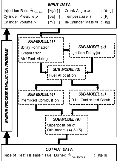
4.1 Model Description ... 31

4.1.1 Inputs & Outputs ... 32

4.1.2 Evaporation & Spray Formation ... 33

4.1.3 Ignition Delay(s) & Fuel Allocation ... 34

4.1.4 Pre-Mixed Combustion ... 35

4.1.5 Diffusion Controlled Combustion ... 36

4.1.6 Parameters ... 37

4.2 Model Parameter Sensitivity Study ... 37

4.3 Comparative Algorithm Study ... 40

4.3.1 Basic Setup ... 40

4.3.2 Algorithm Performance ... 41

4.3.3 Stochastic Initialization & Evolution ... 42

4.3.4 Summary ... 43

4.4 Model Study on Different Engine Sizes ... 43

4.4.1 “Heavy-Duty” Diesel ... 43

4.4.2 “Automotive” Diesel ... 47

4.4.3 “Marine” Diesel ... 49

4.5 Advanced Fuels Survey ... 51

4.6 Conclusions ... 53

5 EMISSIONSOF NITROGEN OXIDE ... 55

5.1.2 Variable Virtual Combustion Zones ... 56

5.1.3 Reaction Mechanism ... 57

5.1.4 Kinetics of NO Formation ... 58

(13)

6 SOOT EMISSION ... 67

6.1.2 “Two Step - Two Zone” Approach ... 68

7 ENGINE PROCESS SIMULATIONS ... 77

7.1 Setup ... 77

7.2 Simulations ... 78

7.2.1 Cylinder Pressure and Temperature ... 78

7.2.2 Combustion Characteristics ... 80

7.2.3 Emissions ... 82

8 ARTIFICIAL NEURAL NETWORKS_...85

8.1 Comparative Study Setup ... 85

8.2 Rate of Heat Release ... 85

8.3 Nitrogen Oxide & Soot Emissions ... 89

9 CONCLUSIONSAND OUTLOOK ... 95

9.1 Summary & Conclusions ... 95

9.2 Outlook ... 96

REFERENCES ... 99

A APPENDIX ... 107

A.1 Operating Conditions ... 107

A.1.1 “Automotive” Diesel ... 107

A.1.2 “Heavy-Duty” Diesel ... 109

A.1.3 “Marine” Diesel ... 111

A.2 Kinetics of NO Formation ... 112

A.3 Correlation & Linear Regression Statistics ... 113

A.4 Cylinder Pressures ... 114

(14)

(15)

L

IST

OF

F

IGURES

1 INTRODUCTION

2 STATE-OF-THE-ART

Fig. 2.1 Control Volume as Used in Single-Zone Cylinder Models... 6 Fig. 2.2 Model of an Artificial Neuron With Interconnections ... 10 Fig. 2.3 Schematic Diagrams of (a) Multi-Layer Feedforward Neural Network and

(b) Simple Recurrent Neural Network... 11 Fig. 2.4 Iterative Optimization Scheme of Optimizer & Analyzer... 14

3 APPROACHESAND EQUIPMENT

Fig. 3.1 Modeling/Optimization Scheme ... 18 Fig. 3.2 Polymer Electrolyte Fuel Cell Modeling:

(a) Sketch of a Single Plate Fuel Cell, (b) Comparison Plot between

the Experimental and Simulated Current-Voltage Characteristics ... 19 Fig. 3.3 Artificial Neural Network Scheme ... 20 Fig. 3.4 Error Objective Function: (a) Standard Least Square Error (LSE),

(b) LSE Including Tolerance Value ... 23 Fig. 3.5 Recombination Mechanisms: (a) Intermediate, (b) Extended Line

Recombination (According to [76])... 24 Fig. 3.6 Examples of Injection Profiles (Rate of Fuel Injected):

(a) Automotive Split Injection Timing and Injection Profile,

(b) Measured Heavy-Duty Single Injection Profile... 28

4 RATEOF HEAT RELEASE

Fig. 4.1 Phenomenological Rate of Heat Release (ROHR) Model ... 31 Fig. 4.2 ROHR Characteristics: (a) Integral and (b) Detailed Premixed & Diffusion

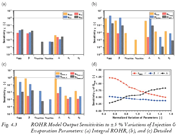
Controlled Combustion Characteristics ... 32 Fig. 4.3 ROHR Model Output Sensitivities to ± 5 % Variations of Injection &

Evaporation Parameters: (a) Integral ROHR, (b), and (c) Detailed Premixed and Diffusion Controlled Combustion Characteristics.

(d) Sensitivity of Q_max to ± 50 % Variations in c_SMD, β, and Λ... 39 Fig. 4.4 Comparison of Experimental and Numerical ROHR Characteristics for

the CMA-ES Algorithm Model Calibration: (a) Sequential Operating Conditions Plot, (b) 1-to-1 Scatter Plot... 40 Fig. 4.5 Comparison of the 4 Algorithms Used for the ROHR Model:

(a) Performance Plot, (b) 1-to-1 Scatter Plot (Best vs. Worst Algorithm) ... 41 Fig. 4.6 Comparative Algorithm Study Statistics: (a) Person’s Correlation

(16)

(a) Error vs. # Function Evaluations (b) Single Parameter Variation ... 43

Fig. 4.8 Heavy-Duty Diesel ROHR Model Calibration & Verification: (a) Sequential Operating Conditions Plot, (b) 1-to-1 Scatter Plot... 44

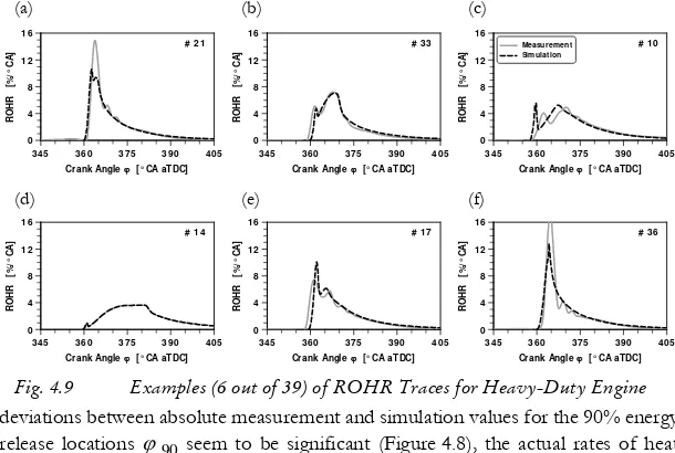
Fig. 4.9 Examples (6 out of 39) of ROHR Traces for Heavy-Duty Engine ... 45

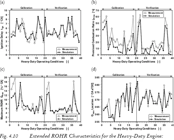
Fig. 4.10 Extended ROHR Characteristics for the Heavy-Duty Engine: (a) Ignition Delay, (b) Premixed Combustion Ratio, (c) Maximum ROHR and (d) Location of Maximum ROHR ... 46

Fig. 4.11 Automotive Diesel ROHR Model: Calibration & Verification... 47

Fig. 4.12 Automotive Diesel Operating Conditions With Pilot- and Main-Injection Pulses: (a) # 3, (b) # 25... 48

Fig. 4.13 Automotive Diesel ROHR: Heavy-Duty Model Blind Try ... 48

Fig. 4.14 Marine Diesel ROHR Model Calibration & Verification (a) Sequential Operating Conditions Plot, (b) 1-to-1 Scatter Plot... 50

Fig. 4.15 Marine Diesel Engine ROHR Model: (a) Blind Try, (b) Adjusted ... 50

Fig. 4.16 Marine Engine Comparison of Three Model Parameter Sets: (a) Pearson’s Correlation Coefficient & Linear Regression Slope, (b) Linear Regression Intercept ... 51

Fig. 4.17 Heavy-Duty Advanced Fuels ROHR Model Characteristics: (a) Calibration/Verification Operating Conditions Plot, (b) 1-to-1 Scatter Plot, (c) Fuel Operating Conditions Plot, (d) Model Errors... 52

Fig. 4.18 Heavy-Duty Advanced Fuels Blind Try ROHR Characteristics: (a) Fuel Operating Conditions Plot, (b) Model Errors ... 53

5 EMISSIONSOF NITROGEN OXIDE Fig. 5.1 Variable representative air/fuel ratio function and associated in-cylinder temperature trace for NO formation... 56

Fig. 5.2 Operating Condition Specific Variations of NOx Model Sensitivities: (a) Point of Discontinuity Combustion Progress Parameters, (b) NO Formation Mechanism Reaction Rate Constants ... 59

Fig. 5.3 Mean (Operating Condition Averaged) NO_x Model Sensitivities: (a) Normalized Variations of λend, cROHR, andζend, (b) ± 5 % Step Size Parameter Variations... 60

Fig. 5.4 Heavy-Duty Diesel NO_x Model Calibration & Verification: (a) Sequential Operating Conditions Plot, (b) 1-to-1 Scatter Plot... 60

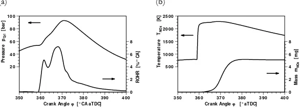
Fig. 5.5 Heavy-Duty Single Operating Condition: (a) Pressure History and ROHR, (b) Representative Temperature and Mass of Nitric Oxide ... 61

Fig. 5.6 Automotive Diesel NO Model: Calibration & Verification ... 62

Fig. 5.7 Automotive NO Emissions: Heavy-Duty Model Blind Try ... 62

Fig. 5.8 Marine Diesel NO Model: Calibration & Verification... 63

(17)

6 SOOT EMISSION

Fig. 6.1 Representative Heavy-Duty Engine Operating Condition: (a) ROHR,

(b) Soot Formed, Oxidized and Total Mass of Soot Histories ... 68

Fig. 6.2 Equivalence Ratio - Temperature Map for Soot Formation: (a) Original Akihama et al [2], (b) Mathematical Approximation ... 69

Fig. 6.3 Operating Condition Specific Sensitivities: (a) Oxidation Activation Temperature TA.oxand Scaling Factor cox, (b) Soot Model Mean Sensitivities for ± 5 % Step Size Parameter Variations ... 70

Fig. 6.4 Heavy-Duty Diesel Soot Model Calibration & Verification: (a) Sequential Operating Conditions Plot, (b) 1-to-1 Scatter Plot ... 71

Fig. 6.5 Automotive Diesel Soot Model Calibration & Verification... 72

Fig. 6.6 Automotive Soot Model: Variation of Engine Load... 73

Fig. 6.7 Automotive Soot Emissions: Heavy-Duty Model Blind Try... 73

Fig. 6.8 Marine Diesel Soot Model Calibration & Verification ... 74

Fig. 6.9 Marine Soot Emissions: Heavy-Duty Model Blind Try ... 75

7 ENGINE PROCESS SIMULATIONS Fig. 7.1 Engine Process Simulation Comparative Study Setup ... 77

Fig. 7.2 Comparison of Cylinder Pressures and ROHRs (left side), Burned Gas and Mean Temperatures (right side) for Three Selected Heavy-Duty Diesel Operating Conditions; (a) # 2, (b) # 5, and (c) # 15 ... 79

Fig. 7.3 Comparison of Engine Process Simulation Characteristics: (a) Maximum Pressure and Location of Maximum Pressure, (b) Maximum Temperature and Maximum Mean Temperature ... 80

Fig. 7.4 Comparison of Cylinder Pressures and ROHRs (left side), Burn and Mean Temperatures (right side) for Operating Condition # 9 ... 81

Fig. 7.5 Comparison of Engine Process Simulation Characteristics (left side: Absolute Values, right side: According Relative Errors): (a) Maximum Pressure and Maximum Mean Temperature (b) Exhaust Pressure and Exhaust Temperature... 81

Fig. 7.6 Comparison of Maximum Pressure Increase and Indicated Efficiency (left side: Absolute Values, right side: According Relative Errors)... 82

Fig. 7.7 Comparison of Nitrogen Oxide Emissions (left side: Absolute Values, right side: According Relative Errors)... 82

8 ARTIFICIAL NEURAL NETWORKS Fig. 8.1 Comparison of Simulation Schemes (ANN vs. Modeling)... 85

Fig. 8.2 Training vs. Verification: Overfitting Criteria ... 85

Fig. 8.3 Heavy-Duty Diesel ROHR ANN Training & Verification: (a) Sequential Operating Conditions Plot, (b) 1-to-1 Scatter Plot ... 86

Fig. 8.4 Heavy-Duty ROHR ANN: Training vs. Verification... 87

(18)

(a) Artificial Neuronal Network, (b) Phenomenological Modeling ... 88 Fig. 8.7 Comparison of Blind Try Marine Diesel Engine ROHR Simulations:

(a) Artificial Neuronal Network, (b) Phenomenological Modeling ... 89 Fig. 8.8 Heavy-Duty Diesel Emissions ANN Training & Verification:

(a) Nitrogen Oxide Emissions, (b) Soot Emissions ... 90 Fig. 8.9 Marine Diesel Nitrogen Oxide Emission Simulation: (a) ANN

Sequential Operating Conditions Plot, (b) ANN 1-to-1 Scatter Plot, (c) ANN Blind Try, (d) Phenomenological Modeling Blind Try... 91 Fig. 8.10 Automotive NO Emissions: (a) Measurements, (b) ANN Simulation... 91 Fig. 8.11 Automotive NO Emissions: (a) 1-to-1 Plot of Training and Verification

Operating Conditions, (b) NO Emission Residuals ... 92

9 CONCLUSIONSAND OUTLOOK

A APPENDIX

Fig. A.1 Comparison of Measured and Numerical Cylinder Pressures for Six Selected Heavy-Duty Diesel Operating Conditions;

(19)

L

IST

OF

T

ABLES

1 INTRODUCTION

2 STATE-OF-THE-ART

Tab. 2.1 Representative ANN Based Diesel Engine Modeling Studies ... 12

3 APPROACHESAND EQUIPMENT Tab. 3.1 Computational Setup ... 21

Tab. 3.2 Artificial Neural Network (ANN) Characteristics ... 22

Tab. 3.3 Objective Functions used for the Model Calibration ... 23

Tab. 3.4 Genetic Algorithm Characteristics ... 24

Tab. 3.5 Evolutionary Algorithm Characteristics ... 25

Tab. 3.6 CMA Evolutionary Strategy Characteristics ... 25

Tab. 3.7 MATLAB GADS Toolbox Characteristics ... 26

Tab. 3.8 Engine and Injection System Specifications ... 27

Tab. 3.9 Overview of Operating Condition Ranges (Minimum .. Maximum) ... 27

Tab. 3.10 Approximate Values of Errors for the Heat Release Analysis Based on In-House Experience 29 4 RATEOF HEAT RELEASE Tab. 4.1 ROHR Model Parameters ... 38

Tab. 4.2 Heavy-Duty Engine ROHR Model Statistics ... 44

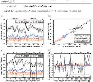
Tab. 4.3 Automotive Engine ROHR Model Statistics for the EA Optimized and the Heavy-Duty Blind Try Case 49 Tab. 4.4 Advanced Fuels Properties ... 52

Tab. 4.5 Heavy-Duty Advanced Fuels ROHR Model Statistics for the EA Optimized and the Heavy-Duty Blind Try Case 54 5 EMISSIONSOF NITROGEN OXIDE Tab. 5.1 Nitrogen Oxide Emission Model Parameters ... 57

Tab. 5.2 Heavy-Duty Engine Calibration & Verification Statistics ... 61

Tab. 5.3 Automotive Engine: Optimized vs. Blind Try Statistics ... 63

Tab. 5.4 Marine Engine Optimized vs. Blind Try Statistics ... 64

6 SOOT EMISSION Tab. 6.1 Soot Emission Model Parameters ... 69

Tab. 6.2 Heavy-Duty Soot Model: Calibration & Verification Statistics ... 72

Tab. 6.3 Variation of Engine Load Operating Condition Data ... 73

Tab. 6.4 Automotive Optimized vs. Blind Try Soot Model Statistics ... 74

(20)

Tab. 7.1 GT-Power Characteristics ... 78

Tab. 7.2 Selected Operating Conditions Specifications (c.f. Figure 7.2) ... 78

8 ARTIFICIAL NEURAL NETWORKS Tab. 8.1 Heavy-Duty ROHR ANN: Training vs. Verification ... 87

Tab. 8.2 Heavy-Duty Engine Pearson’s Correlation Coefficients r ... 87

Tab. 8.3 Marine Engine Pearson’s Correlation Coefficients r ... 88

Tab. 8.4 Heavy-Duty Diesel Specific Soot Emission Details ... 90

9 CONCLUSIONSAND OUTLOOK A APPENDIX Tab. A.1 Automotive Diesel Operating Conditions ... 107

Tab. A.2 Heavy-Duty Diesel Operating Conditions ... 109

Tab. A.3 Heavy-Duty Advanced Fuels Survey Operating Conditions ... 110

Tab. A.4 Marine Diesel Operating Conditions ... 111

Tab. A.5 Rate Constants for the NO Formation Mechanism ... 112 Tab. A.6 Comparative Algorithm Study Statistics:

(r) Pearson’s Correlation Coefficient, (m) Linear Regression Slope, and (b) Linear Regression Intercept 113 Tab. A.7 Marine Diesel Engine ROHR Model Statistics for the EA Optimized,

(21)

N

OMENCLATURE

Latin Variables and Symbols

A Area m2

b Linear regression intercept

-c Scaling factor, velocity, speed - , m/s, m/s

d Diameter m

f, F Function, Allocation function, time delay function

-H Heating Value MJ/kg

k Kinetic energy, reaction rate constants m2/s2,

-l Length m

m Mass, linear regression slope kg,

-n, N Number

-p Pressure Pa

Q Energy, Rate of Heat Release (ROHR) J, J/°CA

r Pearson’s correlation coefficient

-s Speed m/s

t, T Time, Temperature s, K

u Velocity m/s

V Volume m3

x Model parameters

-y Model output characteristics

-Re Reynolds number

-# Number

-Greek Variables and Symbols

β Evaporation rate

-Δ Difference

-ζ Burned mass fraction

-λ, Λ Air/fuel (equivalence) ratio

-ξ Ratio

-η Efficiency

-ρ Density kg/m3

τ Characteristic time s

φ Fuel/air (equivalence) ratio

-ϕ Angle °

(22)

-0 Start, steady-state condition

10 10 %

50 50 %

90 90 %

A Activation

AF Air/Fuel mixture

Chem Chemical

Comb Combustion

Cyl Cylinder

Del Delay

Diff Diffusion (controlled combustion)

e Equilibrium

EO Exhaust Valvle Open

Evap Evaporation

Exh Exhaust

form Formation

g Background

i i th Element

Inj Injection

lam Laminar

max Maximum

meas Measurement

obj Objective

oc Operating condition

ox Oxidation

Prmx Premixed (combustion)

ref Reference

s Soot

sim Simulation

st Stochiometric

tot Total

turb Turbulent

(23)

Abbrevations

ANN Artificial Neural Network

aTDC after Top Dead Center (gas exchange TDC = 0 [°CA])

B60 Diesel-Butylal Blend (60 % Butylal by Mass)

CA Crank Angle

CMA-ES Covariance Matrix Adaption Evolutionary Strategy

CMC Conditional Moment Closure

CPU Central Processing Unit

DI Direct Injection

DNS Direct Numerical Simulation

DoE Design of Experiments

E13 Water-in-Diesel Fuel Emulsion (13 % Water by Mass)

E21 Water-in-Diesel Fuel Emulsion (21 % Water by Mass)

EA Evolutionary Algorithm

EGR Exhaust Gas Recirculation

EP Evolutionary Programming

EPA U.S. Environmental Protection Agency

GA Genetic Algorithm

GADS Genetic Algorithm & Direct Search

HCCI Homogeneous Charge Compression Ignition

IC Internal Combustion

JANAF Joint Army - Navy - Air Force

LAV Aerothermochemistry and Combustion Systems Laboratory

LES Large Eddy Simulation

LTC Low Temperature Combustion

NIST U.S. National Institute of Standards & Technology

PM Particulate Matter

PAH Polycyclic Aromatic Hydrocarbons

RANS Reynolds-Averaged Navier-Stokes

R&D Research and Development

ROHR Rate of Heat Release

s.f. Scaling Factor

SMD Sauter Mean Diameter

SOC Start Of Combustion

SOI Start Of Injection

(24)

(25)

1

I

NTRODUCTION

More than a century after the first simple petrol engine was cranked, the technology which mobilized mankind on land, sea and in the air is on the edge of a period of new developments. There might not be a change in the basic principles of internal combustion engines, but the way the future engines are going to operate will be clearly different from the ones a decade, never mind a hundred years, ago.

Even though the major advances will be electronics empowered by microchips, the pace of this change has mainly been - and will continue to be - forced by con-sumption, emission and emotion (i.e. power output) requirements. In a world where client satisfaction and time to market are major factors, testing and simulation have become increasingly important.

1.1 Motivation and Objectives

Whereas numerical simulations were often restricted to experimental data post-pro-cessing in the past, the most stimulating factor in modern internal combustion engine research and development is the complementary interaction of advanced experimental and computational investigations. Even with the sophistication, wide variety and accuracy of the experimental methods available, the advantages of the computational methods, such as the unbounded data processing and analysis (i.e. potentially full resolution in time, space and species), the time and cost effectiveness, and the prediction capabilities, still persist.

While experimental studies are needed in order to calibrate and verify numerical simulations, computational investigations are required to interpret and complete experimental results. Facing both the exponential increase in IC engine complexity (e.g. Common-Rail direct injection, variable valve train actuation, etc.), and the strin-gent time and cost conditions in the global markets, integrated experimental and computational approaches are in great demand [17][37][80].

(26)

1.2 Common-Rail DI Diesel Engines

Despite the significant contributions to local and global air quality problems, as well as the (potential) health effects, commercial applications are almost exclusively pow-ered by direct injection diesel engines. In addition, due to the high efficiency, supe-rior drivability, low life-cycle costs, the share of diesel powered passenger cars in western Europe increased from 13.8 % in 1990 to 48.2 % in 2004 [1].

In order to control/reduce the negative impacts on the environment, emission regulations specify and enforce the maximum amount of pollutants allowed to be emitted by an internal combustion engine. For common diesel engines, generally the particulate matter (PM)1, the nitrogen oxide (NO_x)2, the hydrocarbons (HC), and the carbon monoxide (CO) emissions are regulated, whereas the carbon dioxide (CO₂) emissions for example are subject to voluntary agreements between adminis-trations and manufacturers.

Facing the increasingly stringent emission regulations, major engine research and development focuses on the simultaneous reduction of fuel consumption and exhaust emissions of diesel engines by combustion and cycle efficiency improve-ments [45]. According to [10], the various technologies developed and implemented in modern diesel engines can be classified - in a non exhaustive list - as follows:

• FUEL INJECTION AND AIR MANAGEMENT

variable-rate fuel injection systems (e.g. Common-Rail), exhaust gas recircu-lation, variable nozzle/geometry turbocharger, two-stage turbocharging, four-valve cylinder heads, variable swirl, variable valve train actuation, etc.

• FUEL COMPOSITION MODIFICATIONS

low sulphur fuels, water-in-diesel fuel emulsions, oxygenated and hydrogen enriched fuels, etc.

• EXHAUST GAS AFTERTREATMENT

oxidation catalysts, diesel particulate filters, nitrogen oxides adsorber cata-lysts, selective catalytic reduction systems, etc.

• COMBUSTION CONCEPT

Homogeneous Charge Compression Ignition (HCCI), Low Temperature Combustion (LTC), etc.

1. Particulate Matter (PM) - both solid and liquid particles of 1 nanometre to 100 micrometres in diameter suspended in the air. IC engine PM emission mainly consist of elemental carbon (soot), unburned fuel (hydrocarbons), and various acids, with a soot content that varies from 25 % to 95 % (depending on the fuel, operating condition and type of engine used) [3].

(27)

Common-Rail DI Diesel Engines

1.2.1 Combustion Analysis and Modeling

Given that in engineering “modeling a process” has become a synonym for develop-ing and usdevelop-ing an appropriate combination of assumptions and equations that permit critical features of a process to be analyzed [44]. Internal combustion engine models thus range from zero-dimensional empirical model, to three-dimensional computa-tional reactive fluid dynamic models.

An experimental combustion analysis generally includes the interpretation of global engine operating characteristics, such as performance/efficiency measures and exhaust emissions, as well as time resolved temperature and (in-cylinder) pres-sure data.

1.2.2 Exhaust Emissions

Diesel exhaust is a complex mixture of gases, vapors, liquid aerosols and substances made up of particles (i.e. fine particles), that has the potential to cause a range of seri-ous health problems. Despite the controversy about the epidemiology studies used to develop health risk assessments of diesel exhaust, long-term/chronic inhalation exposure is likely to pose a lung cancer hazard to humans and short-term/acute exposures can cause irritation and inflammatory symptoms [21].

Among the more than 40 substances emitted by diesel engines that are listed as hazardous air pollutants by the U.S. Environmental Protection Agency (EPA), the nitrogen oxide and particulate matter (soot) emissions are the most important ones. Whereas the nitrogen oxide emissions (along with unburned hydrocarbons and sun-light) make for the formation of ground-level ozone1 and contribute to the forma-tion of acid rain, particulate matter emissions are mainly associated with the serious health effects mentioned above.

1.2.3 Optimization

During the IC engine design process, optimization methods are used for example, to calibrate numerical models [100], to reduce engine exhaust emissions in automated test-bed systems (i.e. electronic control unit calibration) [95], or to find the best fuel/ propulsion systems in life cycle analysis studies [64]. The optimization techniques employed range from gradient-free methods, such as evolutionary algorithms or coordinate strategies, to first and second-order gradient methods, such as conjugate gradient or Newton’s method (c.f. Section 2.4 and [69]).

(28)

1.3 Approach

To describe the manner in which the goals outlined in Section 1.1 were attained, this thesis is structured in three parts. After a detailed survey on the current state-of-the-art IC engine modeling techniques, as well as Artificial Neural Network (ANN), Design of Experiments (DoE), and the application of optimization techniques in IC engine research and development (Chapter 2), both the model/knowledge based and the black-box modeling approach, as well as the computational and experimen-tal setup are presented in Chapter 3.

In the second part of this thesis, a thorough investigation of the phenomenological model/knowledge based approach is given. Starting with a phenomenological Common-Rail DI diesel engine Rate Of Heat Release (ROHR) model in Chapter 4, consistent models for the simulation of nitrogen oxide and soot exhaust emissions are given in Chapters 5 and 6, respectively. In addition to the model description and parameter studies in the first two sections of Chapters 4 to 6, each model is applied to three distinct engines - an automotive, a heavy-duty and a marine diesel engine - in order to evaluate the respective model generalization capability. In addition to these main investigations, which are conducted for all three models, both a compar-ative algorithm study and an advanced fuels investigation are used to further evaluate the ROHR model (Chapter 4). To conclude the model/knowledge based approach part, Chapter 7 presents the application of the derived phenomenological models in various engine process simulations.

(29)

2

S

TATE

-

OF

-

THE

-A

RT

The subsequent sections are intended to give an overview of the classic modeling approaches for internal combustion engines and two potential alternatives; the arti-ficial neural network (ANN) and design of experiments (DoE) approaches. An out-line on the various optimization techniques in engineering closes the chapter.

2.1 Internal Combustion Engine Modeling

The manifold tasks and applications in engine research & development (R&D) have led to various types of combustion engine simulation models. Ranging from fast and rather approximate models to exhaustive but time-consuming models, a classifica-tion into three major categories is commonly used [16][19]. Depending on the inten-tion of the classificainten-tion, the categories are either dimensional (zero-, quasi- and multi-dimensional) or complexity level based (empirical/thermodynamic, phenome-nological and detailed/complex).

2.1.1 Empirical or Thermodynamic Models

Derived from the first law of thermodynamics, mass balances and experimentally obtained correlations, this type of models just accounts for only temporal variations (ordinary differential equations), i.e. spatial variations in composition and thermody-namic properties are neglected. Typically, the whole combustion chamber is mod-eled as a homogeneously mixed zone (a.k.a. single-zone combustion models). Given these simplifications, the models are computationally efficient and easy to handle, but fail to resolve local phenomena, such as fuel spray interaction, turbulence struc-ture and emission formation.

Single-Zone Cylinder Model

Defining the entire combustion chamber as control volume (c.f. Figure 2.1) and applying the conservation law for mass and energy (i.e. the first law of thermody-namics), results in the two governing equations for open thermodynamic systems:

(2.1)

(2.2)

(presuming all flows directed into the control volume have positive signs). dm_cyl

dt

--- dmk dt --- dmin

dt ---=

k

∑

dmexh

dt

--- dmfuel dt

--- dmbb dt

---+ + +

=

dU_cyl dt

--- dQw dt

--- dQchem dt

--- p_cyldVcyl dt

---– h_kdmk

dt

---k

∑

+ +

(30)

[image:30.421.53.342.59.230.2]

Fig. 2.1 Control Volume as Used in Single-Zone Cylinder Models In order to solve the equations for the change in internal energy of the control vol-ume, a series of sub-models are required, e.g. for the mass fluxes (gas exchange, fuel injection and blow-by), mechanical work (friction), heat transfer to the combustion chamber walls, ignition delay and the rate of heat release. Furthermore, to link the change of internal energy to changes in temperature and pressure, thermodynamic gas property correlations, such as the polynomials developed by Zacharias [108] or the NIST-JANAF tables [22] are needed.

Applications & Examples

Single-zone thermodynamic models have been, and still are frequently used in inter-nal combustion engine R&D, specifically for common investigations, such as the analysis of in-cylinder pressure data, transient powertrain simulations or control engineering applications. Therefore, this class of models comprehends numerous modeling approaches.

• HEAT TRANSFER

Directly derived from experimental correlations there are single equation models by Nusselt [71] and Eichelberg [28]. The widely used Woschni for-mula [106] - which is based on an analogy between the in-cylinder flow pat-tern in a combustion engine and the turbulent flow patpat-tern in a circular tube - is another good example of this type of model.

• RATE OF HEAT RELEASE

Generally there is no detailed modeling of physical and chemical processes in single-zone models. Hence, mathematical “substitution” functions, derived from analytical theory and measurement approximations, such as the Vibe combustion profile [98], the polygon-hyperbola profile [84] or the two equa-tion analytical profile [39] are widely used.

U m

cyl cyl

control volume dQw

dWt

hbb

dmbb

dQ h dm

chem fuel

fuel

hin

dmin

hexh

(31)

Internal Combustion Engine Modeling

• EMISSIONS

Based on the in-cylinder mean temperature data of a single-zone model, Schröer [85] derived an empirical correlation (i.e. there is no chemical reac-tion scheme used) to model engine-out emissions of nitrogen oxide. As for soot emissions, most global one-step equation models belong to this class of model (e.g. Khan et al. [57] or Lee [63])

2.1.2 Phenomenological Models

Phenomenological models aim to strike a balance between computational require-ments and model accuracy. In order to overcome the deficiencies of the empirical models in handling local phenomena, the control volume (i.e. the combustion cham-ber) is typically divided into multiple zones characterized by different temperatures and compositions. The zoning is thereby either done sequentially, i.e. along a given time axis - such as the two-zone models by Hohlbaum [49] and Rakopoulos et al. [79], and the n-zone model by Weisser et al. [101] - or geometrically, i.e. in space - such as the “packages” model by Hiroyasu et al. [47].

Using simplified yet physically and chemically coherent models to capture the underlying local processes (i.e. spray atomization, fuel evaporation, air entrainment, ignition, etc.) phenomenological models allow for both qualitative and quantitative predictions of pollutant emissions and rates of heat release. Given the simplistic spa-tial resolution (the number of zones accounted for is usually in the range of two up to a few dozen), the absence of the Navier-Stokes momentum equation, as well as the spatial averaging of the turbulent flow field, these models are not able to account for example for the effects of changes in combustion chamber geometry, such as different bowl shapes, or complex interactions among different zones.

Applications & Examples

Phenomenological models are typically applied in experimental data analysis, optimi-zation of control variables, or simulations over entire engine operating maps, to bridge the gap until detailed three-dimensional models become computationally affordable. Combining low computing times (generally of the order of seconds for one operating condition) and reasonably accurate predictions for global combustion parameters, these models are best suited for conceptual studies.

• HEAT TRANSFER

(32)

overall heat flux is strongly dependent on the local conditions, most of the models divide the combustion chamber into sections by merging similar conditions [29][86].

• RATE OF HEAT RELEASE

Given the tight coupling of the physical and chemical processes present in combustion engines (e.g. fuel evaporation and air entrainment), common rate of heat release models consequently consider the whole range of in-cyl-inder processes. Various sub models are used to represent the injection, air entrainment, ignition, and combustion processes.

Although the aforementioned approaches may differ, they share the same phenomenological concept; the breakdown of the combustion into kineti-cally controlled (“premixed”) and mixing-controlled (“diffusion”) compo-nents. Recent technical advances in multiple pulse injection systems have resulted in substantial work on extending the models to account for different injection strategies [7][67][91].

• EMISSIONS

Based on the (extended) Zeldovich reaction mechanism for the formation of nitric oxide, models for both a “quasi” two-zone approach [42] and an n-zone approach [102] have been extensively used. Numerous versions of a two step equation approach (formation and oxidation) have been proposed to model soot emissions [48][88]. Additionally, there has also been work on integrated approaches for the rates of heat release, soot and NO_x emission modeling (e.g. [14][34][93]).

2.1.3 Detailed or Complex Models

Akin to empirical and phenomenological models, the governing principles for detailed/complex models are the conservation of mass, energy and momentum (a.k.a. Navier-Stokes equation). Solving these conservation laws in time and (three-dimensional) space results in a set of partial differential equations (PDEs). Further-more the chemistry processes prevailing in combustion, as well as the interaction between the chemistry and the fluid mechanics described in three-dimensional Navier-Stokes equations increase the complexity (i.e. the numerical stiffness) of the present models.

(33)

Internal Combustion Engine Modeling

RANS simulations are currently employed in a majority of the cases for the sake of simplicity and available computation time [8], whereas predominantly LES and DNS simulations are used in fundamental research studies [33][61].

Owing to the limited understanding and the complexity of the reaction chemistry at a fundamental level, there is considerable activity in this field of research, includ-ing studies on hydrocarbon reaction mechanisms [9] or turbulence-chemistry inter-actions [107].

Applications & Examples

Compared to empirical and phenomenological models, the generality of detailed/ complex models makes it possible to comply with almost any kind of problem. Depending on the intention, and hence the level of sophistication, the models are commonly used to gain insight into the governing processes, provide information of local in-cylinder phenomena or evaluate new combustion technologies.

• HEAT TRANSFER

Gosman and Watkins applied computational fluid dynamic simulations for turbulent in-cylinder flows including a one-dimensional gas-wall heat trans-fer model [36]. Given the present LES and DNS turbulence models avail-able, the model accuracy is no longer restricted in terms of the turbulent flow field resolution.

• RATE OF HEAT RELEASE / COMBUSTION

Focusing on the combustion itself, numerous approaches, such as the char-acteristic time scale models by Magnussen et al. [65], the flamelet approach by Peters et al. [76] or the Conditional Moment Closure (CMC) model by Bilger et al. [12] exist. Details about the advantages and disadvantages of each of these models, as well as a general survey on multidimensional com-bustion modeling are given by [92].

• EMISSIONS

As the thermal nitric oxide formation based on the Zeldovich mechanism is included in most commercially available engine simulation codes, the main emphasis in nitrogen oxide emission studies is on prompt NO, NO₂ and N₂O formation, and catalytic removal processes (e.g. Miller [68]).

(34)

2.2 Artificial Neural Networks

Inspired by biological nervous systems - such as the human brain, where informa-tion is transmitted and stored in groups of interconnected neurons1 - Artificial Neural Networks (ANNs) employ clusters of small and simple information process-ing units (a.k.a. artificial neurons) to mimic the natural learnprocess-ing process and thereby acquire knowledge.

Similar to the human brain, ANNs operate like “black box” models, as they do not require detailed information about the basic system being observed. ANNs “learn” the relationship between input and output parameters by “studying” given data, and “store” the knowledge in the interconnections, or rather the associated weights (akin to the synapses efficacy in biological neural systems).

Basic Structures & Definitions

In a simplified model of an artificial neuron, the given inputs are weighted, added up and passed through an activation function (e.g. a threshold, linear or sigmoid2 func-tion) to produce an output signal, as shown in Figure 2.2. Combining several artifi-cial neurons in a network architecture, similar neurons are generally arranged in layers that are labeled as input, hidden and output layers (a.k.a. multi-layer network architecture). During the training mode of an ANN, an appropriate learning algo-rithm (e.g. backpropagation3) is used to modify the interconnection weights such that, given selected inputs, the network attempts to produce the desired outputs.

Fig. 2.2 Model of an Artificial Neuron With Interconnections

1. Neuron - primary cell of the nervous system, consisting of a cell body, the axon (single long activa-tion fiber out of the cell body) and multiple dentdrites (receptive nerve fibers)

2. Sigmoid - curved in two directions, viz. shaped like the letter S (c.f. Figure 2.2) 3. Backpropagation - abbreviation for “backwards propagation (of errors)”

x1

x2

xn

xj

wi1

wi2

wij

win

Σ

...

Act ivat ion Funct ionαi

yi= αi(Σxj·wij)

yi

INPUTS

Weight s

Summat ion OUTPUT

x1

x2

xn

xj

wi1

wi2

wij

win

Σ

...

Act ivat ion Funct ionαi

yi= αi(Σxj·wij)

yi

INPUTS

Weight s

(35)

Artificial Neural Networks

Types of Artificial Neural Networks

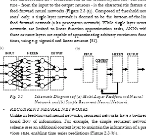
Although the modular design of ANNs allows for numerous network architectures, mainly the feed-forward and the recurrent neural network schemes are used for engi-neering systems [40].

• FEED-FORWARD NEURAL NETWORKS

The unidirectional flow of information in the distinct layered network struc-ture - from the input to the output neurons - is the characteristic feastruc-ture of feed-forward neural networks (Figure 2.3 (a)). Composed of threshold neu-rons1 only, a single-layer network is deemed to be the bottom-of-the-line feed-forward network (a.k.a perceptron network). While single-layer neural networks are limited to linear function approximation tasks, ANNs with three or more layers are capable of approximating arbitrary continuous func-tions, using e.g. sigmoid and linear neurons [51].

• RECURRENT NEURAL NETWORKS

Unlike in feed-forward neural networks, recurrent networks have a bi-direc-tional flow of information. For example, the simple recurrent network scheme uses an additional context layer to maintain the information of a pre-vious state, enabling time series predictions (Figure 2.3 (b)).

Applications

A summary on the numerous applications of ANNs in internal combustion engines, such as emissions and performance modeling, engine controller design and fault diagnosis is given in [52].

Focusing on diesel engine modeling topics only, Table 2.1 lists examples of recent studies including ANNs used in various applications.

1. Threshold Neuron- artificial neuron with a “threshold” activation function, i.e. given normalized inputs and weights, the output is typically 1 or -1 with a threshold value of 0

[image:35.421.72.367.129.402.2]

(a) (b)

Fig. 2.3 Schematic Diagrams of (a) Multi-Layer Feedforward Neural Network and (b) Simple Recurrent Neural Network

. . .

OUTPUT INPUT HIDDEN

. . .

OUTPUT

INPUT HIDDEN INPUT HIDDEN OUTPUT

CONTEXT

OUTPUT

INPUT HIDDEN

(36)

2.3 Design of Experiments (DoE)

The (statistical) Design Of Experiments (DoE) offers a range of procedures and methods for planning experiments, so that it is possible to analyze, predict and opti-mize the influence of one or more input variables on the output variable(s) of an experiment.

According to the “Engineering Statistics Handbook” [70], the key steps in a DoE study are the:

1. SPECIFICATION OF OBJECTIVES & ASSUMPTIONS

depending on the intention of the design1, i.e. whether a comparative (choose between alternatives), screening (identify significant input/output variables) or modeling study is planed

2. SELECTION OF INPUT & OUTPUT VARIABLES

including all relevant but no dispensable variables

3. SELECTION OF EXPERIMENTAL DESIGN

depending on the number of variables and the objectives chosen

AUTHORS TOPIC(S)

Clark et al. [23] exhaust emission modeling (CO2, NOx) based on engine speed & torque (incl. 1st & 2nd derivatives)

De Lucas et al. [24] modeling the influences of fuel specifications (composi-tion, cetane index, etc.) on PM emissions

Delagrammatikas et al. [25] combination of DoE & ANNs for vehicle-level optimi-zation studies (e.g. fuel consumption, acceleration times)

He and Rutland [41] modeling of in-cylinder pressure, temperature, wall heat transfer, NO_x and soot emissions

Hentschel et al. [43] in-car modeling of transient exhaust emissions (opacity, NO_x) with dynamic ANNs (ECU data inputs) Kesgin [56] emission (NO_x) and efficiency modeling Ouenou Gamo et al. [73] exhaust emissions (i.e. opacity) modeling

Papadimitriou et al. [74] automatically selected neural networks for engine cali-bration in control-oriented applications

Traver et al. [96] transient emission modeling (NOx, CO, CO2 and HC) using in-cylinder combustion pressure data

Tab. 2.1 Representative ANN Based Diesel Engine Modeling Studies

(37)

Optimization

4. EXECUTION OF THE DESIGN (EXPERIMENT)

5. DATA CONSISTENCY CHECK WITH ASSUMPTIONS

are the results reproducible?

6. ANALYSIS & MODELING OF THE RESULTS

examine the results for outliers, typographical errors and obvious problems, create the model from the data, check the model residuals and use the results to answer the questions set in the objectives

Using (simple) mathematical functions (a.k.a. regression functions) to model the effects of the input variables on the output of the system, the DoE response surface models differ significantly from other approaches, such as ANNs or phenomeno-logical models. Both ANN and DoE approaches use “black-box” concepts to model the system behavior, and while ANN models are capable of approximating any con-tinuous function describing the input/output correlations, DoE models are not.

Applications & Examples

Despite the limitations in generality, given the structured procedure and the possibil-ity to reduce the number of experiments necessary, DoE approaches are commonly used in industrial applications, such as combustion engine R&D [18]. Examples range from comparative studies of engine components and injection strategies for an automotive DI diesel engine [13], to screening and modeling studies of the in-cylin-der flow field and combustion chamber geometry for a medium-duty DI diesel engine [77].

2.4 Optimization

Optimization can be defined as the search for the best possible solution(s) to a given problem. In general, the n-dimensional optimization problem is expressed by

, (2.3)

where is the parameter vector minimizing1 the (single-)objective function , subject to the equality and inequality constraints given. Additionally, the limits (high/low) for the parameter vector values are defined as , where stands for the lower and for the higher limit respectively.

1. In practice, the optimum is generally defined as the minimum of an objective function. Maximum optimization problems are therefore transformed into minimization problem using max( f(x) ) = -min( -f(x) ).

min(f( )x )

g_i( )x = 0,i= 1,…,p

h_j( )x ≤0, j= 1,…,q

⎩ ⎪ ⎨ ⎪ ⎧

x∈ℜn

f ( ) ℜx ∈ g_i( )x h_j( )x

(38)

Given that in engineering applications, e.g. gas turbine design [20], multiple (con-flicting) objectives have to be optimized, the result of an optimization is a set of “trade-off” solutions (i.e. pareto optimal set1), rather than one single best solution. A mutual comparison of at least two solutions from the pareto set thereby shows, that both of them are better and worse in at least one objective at the same time [97].

Various solutions exist to tackle the optimization problem, most of them sharing the iterative concept of splitting-up the parameter vector estimation (optimizer) and the parameter vector evaluation (analyzer) as in Figure 2.4

Fig. 2.4 Iterative Optimization Scheme of Optimizer & Analyzer The classification of single-objective optimization algorithms is based on whether a method requires information from the objective function’s first and second order derivatives, or only from the objective function. Additionally, a distinction is made between stochastic and deterministic methods. Using information from only the objective function (i.e. direct), in combination with stochastic processes e.g. in the reproduction and variation of the parameter vectors, the evolutionary computation algorithms are classified as direct-stochastic optimization methods. In contrast, the classic coordinate strategy may serve as an example for the direct-deterministic group of optimization methods [69].

2.4.1 “Classic” Methods

In general, the classic algorithms of gradient descent, deterministic hill climbing and purely random search (with no heredity) perform poorly when applied to nonlinear optimization problems. As there exists no algorithm solving for all optimization problems, that on average performs superior to any other algorithm (according to the no-free-lunch theorem [104]), the classic algorithms outperform advanced and complex algorithms in solving linear, quadratic or unimodal problems.

1. Pareto optimality - the parameter vector is pareto optimal if and only if there is no vector

xsuch that for all with at least once strict inequality.

x'∈ℜn

fi( )x ≤fi( )x' i∈{1 2, ,…,n} INITIALIZATION of paramet er vect orx0

EVALUATION (ANALYZER) of a given paramet er vect orxi

ESTIMATION (OPTIMIZER) of an improved paramet er vect orxi+ 1

RESULT TERMINATION?

YES NO

ITERATION INITIALIZATION of paramet er vect orx0

EVALUATION (ANALYZER) of a given paramet er vect orxi

ESTIMATION (OPTIMIZER) of an improved paramet er vect orxi+ 1

RESULT TERMINATION?

YES NO

(39)

Optimization

2.4.2 “Evolutionary Computation” Algorithms

The mutual basis of all regular approaches in evolutionary computation, specifically genetic algorithms, evolution strategies and evolutionary programming, is the imple-mentation of the evolution principle: reproduction, random variation, competition and selection of contending individuals1 in a population2. Thus, the general charac-teristics outlining any evolutionary algorithm are the collective learning process of a population of individuals, the randomized processes intended to model mutation3 and recombination4 and the assignment of a measure of quality or fitness value to an individual [5].

Translated into a pseudo-program-code, the general scheme of an evolutionary algorithm look as follows:

initialize the population evaluate the initial population REPEAT

recombine the individuals to produce an offspring

recombine population

mutate the individuals of the offspring population evaluate the solutions for the offspring population assign a measure of quality to the individuals select the (best) individuals for the next generation UNTIL some convergence criteria is satisfied

Utilizing the size of the parent and offspring population, as well as the character-istics for the recombination, mutation, evaluation and selection processes (also referred to as strategy parameters) as inputs, the evolutionary algorithm iteratively converges towards the optimum solution.

Genetic Algorithms (GAs)

Three features distinguish GAs from other evolutionary algorithms:

• BINARY REPRESENTATION (ENCODING)

Various subsequent implementations of the original GA5 use real-valued representation schemes instead of the bitstring encoding (i.e. the parameter vector consists of 0’s and 1’s only) to be more easily applied to the problem being tackled.

1. Individual - single parameter vector, representing (encoding) a search point in the space of potential solutions to a given problem

2. Population - a pool of individuals

(40)

• PROPORTIONAL (PROBABILISTIC) SELECTION METHOD

Because of the high selective pressure1 associated with it, the probabilistic selection of individuals according to their fitness value runs the risk of pre-mature convergence of a population. That is, the “best” individuals become dominant and hence start to inbreed2.

• CROSSOVER RECOMBINATION

Crossover recombination randomly swaps single values (bits) or segments of the parameter vectors of two dissimilar individuals, aiming to combine the best features from both individuals and thus creating a better offspring. Although most GAs use mutation along with crossover recombination, almost exclusively crossover recombination is used to assure the diversity and broadening of the population.

Evolution Strategies (ESs)

Using normally distributed mutations to modify the real-valued parameter vectors, the emphasis in ESs is equally placed on mutation and recombination as search operators. Moreover, the simultaneous adjustment (extended optimization) of the strategy parameters and the parameter vector itself further distinguishes the ESs from other GAs.

Unlike in GAs, the selection operators in ESs are deterministic and the parent and offspring population sizes usually differ from each other. That is, the number of par-ents is less or equal the number of offspring and thus the worst performing individ-uals (i.e. the ones with the lowest measure of quality) of an offspring generally don’t procreate.

Evolutionary Programming (EP)

Similar to ESs, the EP algorithms use normally distributed mutations and extend the evolutionary process to the strategy parameters as well. Emphasizing mutation while neglecting the recombination of individuals, EP algorithms drop the implicit assumption that the fitness value is linked to parts of the parameter vector, as is usu-ally assumed for GAs and ESs.

Further studies on applications, advantages and disadvantages of the various opti-mization algorithms used in EP are given in [6][30][89], whereas [35][50][60][81] pro-vide the fundamentals for the various approaches.

1. Selective Pressure - probability of the best individual being selected compared to the average prob-ability of selection of all individuals

(41)

3

A

PPROACHES

AND

E

QUIPMENT

After briefly defining the system and introducing the objectives of the study, detailed information on both the “model/knowledge based” and “black-box” approaches are given in the first part of this chapter. The second part subsequently documents the equipment used, i.e. both computer soft-/hardware and the three distinct IC engines and utilized measurement techniques.

3.1 System & Objectives

The combustion of a Common-Rail DI diesel engine, as characterized by the rate of heat release and the nitrogen oxide and soot emissions, serves as a measure for the subsequently described comparative investigation. Given the general engine and operating condition specifications as inputs, the actual ROHR and specific NOx and

soot emissions are defined as outputs.

The objectives of the study are the fast and reliable prediction of the system out-puts for three distinct types of engines, more specifically an automotive, a heavy-duty and a two-stroke marine diesel engine. Additionally, the investigation includes the comparison of two dissimilar approaches for modeling; the “model or knowl-edge based” and “black-box” approaches. As there are at least two optimization sequences necessary to get from initiation to an optimized simulated engine operat-ing map, a concept for the interaction of modeloperat-ing and optimization is derived.

3.2 “Model/Knowledge Based” Approach

The model or knowledge based approach in this context refers to a physical and chemical description of the underlying system, derived from both fundamental theory and phenomenological experience. As stated in the objectives, the description of the system (i.e. the basic models) should allow for fast and reliable predictions of the system outputs. In other words: the models used in this approach need to be as complex as necessary and as simple as possible at the same time. Hence, given the restrictions and requirements, only phenomenological models (c.f. Section 2.1.2, p. 7) are used in this study.

(42)

model calibration thereby significantly affects the outcome of the subsequent search for the system optimum.

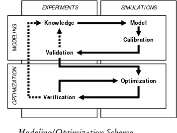
3.2.1 “Modeling/Optimization” Scheme

[image:42.421.110.288.215.349.2]

Based on experience from joint experimental and numerical combustion engine R&D projects, such as [59] and [83], a fundamental modeling and optimization scheme is derived to profit from the mutual advantages of both subjects. Along with the distinction between modeling and optimization, the strict subdivision of exper-imental data into calibration and verification parts thereby assures the formal cor-rectness of the approach. Although the objectives of the two optimization parts in the scheme, the “model calibration” and the “system optimization”, differ, the opti-mization algorithms do not need to be dissimilar.

Fig. 3.1 Modeling/Optimization Scheme

Starting from available (experimental) knowledge of the system, there is an itera-tive process of modeling, calibration and verification to derive an appropriate model of the system. Given an appropriate model, the iteration between the numerical opti-mization and the experimental validation allows for both the optiopti-mization of the system outcome and a profound understanding of the application (Figures 3.1).

3.2.2 Application Examples

As the proposed modeling/optimization scheme by itself is not restricted to diesel engine combustion systems only, it has successfully been applied to other applica-tions using the same procedures, e.g. evolutionary algorithms as optimization method.

EXPERIMENTS SIMULATIONS

M

O

D

E

L

IN

G

O

P

T

IM

IZ

A

T

IO

N

Knowledge Model

Validation

Calibration

Verification

Opt imization

EXPERIMENTS SIMULATIONS

M

O

D

E

L

IN

G

O

P

T

IM

IZ

A

T

IO

N

Knowledge Model

Validation

Calibration

Verification

(43)

“Black-Box” Approach

3.2.2.1 Thermodynamic Modeling

Similar to the approach used to model the nitrogen oxide and soot emissions from Common-Rail DI diesel engines (c.f. Chapters 5 and 6), Lämmle [62] uses the scheme to model knock1 phenomena in SI natural gas engines.

Using computational reactive fluid dynamic simulations of HCCI2 phenomena in diesel engines, Barroso [9] applied the scheme to determine the kinetic parameters for the governing reactions in a hydrocarbon combustion mechanism.

3.2.2.2 Polymer Electrolyte Fuel Cell Modeling

Using evolutionary algorithms for parameter optimization, a phenomenological 1+1 dimensional model for Polymer Electrolyte Fuel Cells (PEFCs) [32] was calibrated according to the modeling/optimization scheme.

Comparing the model calibration accuracy for the global current-voltage charac-teristics of a single plate fuel cell, the modeling/optimization scheme with evolution-ary algorithms exceeds the classic manual model calibration.

3.3 “Black-Box” Approach

The generic term black-box approaches commonly stands for a variety of methods, such as Artificial Neural Networks (ANNs), statistical regression or fuzzy logic models, which do not contain physical or chemical models. The omission of physical or chemical models to describe the interdependence of the system inputs and

out-1. Knock - pressure waves/fluctuations associated with autoignition of a portion of the air-fuel mix-ture ahead of the advancing flame front

2. HCCI - Homogeneous Charge, Compression Ignition

(a) (b)

Fig. 3.2 Polymer Electrolyte Fuel Cell Modeling: (a) Sketch of a Single Plate Fuel Cell, (b) Comparison Plot between the Experimental and Simulated Current-Voltage Characteristics

V

o

lt

a

g

e

[V

]

0. 45 0. 50 0. 55 0. 60 0. 65 0. 70 0. 75 0. 80 0. 85 0. 90

Current [ A]

0 20 40 60 80 100 120 140 160 180 200

Measurement Manual Model Calibrat ion Modeling/ Opt imization Scheme

p_O2, p_H2 = 2 [ bar]

λAir, λH2 = 2 [ -]

(44)

puts is the major advantage and disadvantage of the black-box approaches at the same time. Considering that there is little or no a priori knowledge of the system nec-essary, the approach is best suited for systems where there is a lack of fundamental understanding. Alternatively, given a system where fundamental knowledge on the system behavior is available, black-box approaches tend to be less efficient than model/knowledge based approaches. Partial black-box approaches, a.k.a. grey-box methods1, are one way to compensate for this drawback, using fundamental knowl-edge in the form of phenomenological models where available.

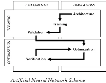
3.3.1 “Artificial Neural Network” Scheme

[image:44.421.110.286.262.401.2]

In the present study an Artificial Neural Network (ANN) scheme is used as an alter-native example to the phenomenological modeling/optimization scheme (c.f. Section 3.2.1). Similar to the modeling/optimization scheme, the ANN process con-sists of two basic phases; network training and system optimization (Figure 3.3). Unlike in the modeling phase of the modeling/optimization scheme though (Figure 3.2), there are generally no iterations needed in the network training phase.

Fig. 3.3 Artificial Neural Network Scheme

Starting from a particular ANN architecture and a set of corresponding input and output data (training data), a learning algorithm modifies the interconnection biases and weights such that the network attempts to reproduce the behavior of the system. Once the network is trained, the subsequent system optimization phase is analog to the one in the modeling/optimization scheme (Figures 3.2 and 3.3).

1. Grey-box methods - systems or modules are defined by external interfaces, as black-box methods, and a partially resolved internal structure based on knowledge

EXPERIMENTS SIMULATIONS

T

R

A

IN

G

O

P

T

IM

IZ

A

T