A spatial approach using imprecise soil data for
modelling crop yields over vast areas
Philippe Lagacherie
a,∗, Durk R. Cazemier
a,
Roger Martin-Clouaire
b, Tom Wassenaar
aaINRA Science du Sol, 2 Place Pierre Viala, 34060 Montpellier Cedex, France bINRA, Biométrie et Intelligence Artificielle, BP27, 31326 Castanet-Tolosan Cedex, France
Received 25 August 1999; received in revised form 10 December 1999; accepted 28 February 2000
Abstract
Estimations of crop yields using process-based crop models are area-limited because quantitative soil data are unavailable over vast areas. The spatial approach proposed in this study incorporates two novel aspects concerning the derivation of soil data feeding the simulation and the modelling of the crop production process. First, the soil parameters required for crop modelling as well as their imprecision were estimated from the qualitative information of a 1:250,000 scale regional soil database by a possibility theory approach, which combines a set of GIS procedures and a constraint satisfaction solver. Second, the initial process-based crop model was made less complex by deriving simple agrotransfer functions from simulations at representative sites located in the studied region. The resulting system estimated the yield expressed as possibility distributions over the region which can be visualised through decision maps. The proposed spatial approach was tested on a hard wheat yield (Triticum durum spp.) estimation in the Hérault-Orb-Libron valley region (Languedoc, France). It proved to provide realistic yet imprecise estimates compared with those obtained for a set of site-crop estimates. The spatial approach allowed the identification of areas in which soil data needed to be improved for obtaining both reliable and informative estimates. These results demonstrated the potential usefulness of the proposed approach for providing reliable soil information for decision making at the regional level. © 2000 Elsevier Science B.V. All rights reserved.
Keywords: Soil map; Available water capacity; Regional scale; Crop model; Imprecision; Possibility theory; Constraint satisfaction problem;
GIS
1. Introduction
Computer simulations of soil water regimes and crop growth are powerful means for quantifying the effects of changing climate conditions or agricultural practices. However, these simulations require a large amount of quantitative soil data which limits their spa-tial application to areas where a dense spaspa-tial sampling
∗Corresponding author. Tel.:+33-4-99-61-25-78;
fax:+33-4-67-63-26-14.
can be undertaken. A spatial approach is needed for extending the simulations to vast areas such as Euro-pean regions.
The common practice for doing this consists in linking crop models to quantitative information pro-vided by soil maps and soil databases (Dumanski et al., 1993; Smaling and Fresco, 1993; Akinremi et al., 1997; Bornand et al., 1998). This type of informa-tion consists in measured soil data from detailed soil profile observations that are assumed to be represen-tative for the delineated mapping units. Crop yield
simulations can then be undertaken by using these input data, if necessary, in combination with pedo-transfer functions (Bouma and van Lanen, 1987). The so obtained results are assumed to be valid for the whole mapping unit, thus allowing easy mapping by classical GIS procedures.
This straightforward approach becomes question-able when yield must be mapped over large areas. Generally, small scale soil maps (<1:250,000) are the only available soil information over such areas. At this scale the mapping units often include several taxonomic units, each of them characterised by a rep-resentative profile. The common practice is to select the representative profile of the dominant taxonomic units which can lead to neglect a substantial part of the mapping unit area (Le Bas et al., 1998). Further-more the taxonomic units of a small scale soil map cannot be reduced to the description of a unique set of parameters measured at a given site because of its high within-unit variability. Resuming, the exclusive use of quantitative information derived from a small scale soil map leads to a misrepresentation of the soil variability of the region. This may have consequences on yield mapping and further decision making.
A possible alternative is to use the qualitative de-scription of the soil taxonomic units (STUs) of a small scale map as input data for crop models. This description provides a more synthetic understanding of the taxonomic units taking into account the entire information collected by the soil surveyor in the field, i.e. soil profiles, auger hole observations and surface features observations. The description of a STU also includes a description of environmental attributes (e.g. geology, land use, slope). If maps of these at-tributes exist for the studied region, the environmental descriptions can be used for estimating the location of each STU within the complex soil mapping units of the 1:250,000 scale soil map.
All this qualitative information, generally based on well-established codification systems (FAO-UNESCO, 1981; Baize and Jabiol, 1995), is now easily avail-able in soil databases (Oldeman and van Engelen, 1993; Bornand et al., 1994; King et al., 1994). This information is, however, still underexploited in yield predictions. The approach presented below estimates crop yields over a region by coupling simulations with the qualitative descriptions of taxonomic soil units of a 1:250,000 soil database. Such coupling is
made through agrotransfer functions derived from a set of crop model simulations undertaken over a set of representative soil climate situations. The proposed approach uses possibility theory for representing and handling the required qualitative information. It was applied within the framework of the EC funded re-search project IMPEL (Rounsevell et al., 1998) for mapping hard wheat yields evolutions with changing climate conditions over a region of 1200 km2located in the Languedoc plain (southern France). This paper focuses on the estimation of wheat yield under actual climate conditions. The climate changes issues dealt in the IMPEL project are detailed in Wassenaar et al. (1999).
2. The spatial approach
2.1. Representing qualitative descriptions of soil taxonomic units by possibility distributions
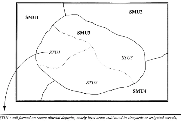
Fig. 1 shows an example of description of STU in a regional soil database. STUs are non-geographic components of soil landscape units (King et al., 1994) delineated in small scale soil maps. The first part of STU description (Fig. 1, in italics) deals with the STU environment whereas the second part is a description of the soil properties which characterise the STU.
Fig. 1. An example of qualitative description of STU in a regional soil database. STU: soil taxonomic units, SMU: soil mapping unit, italic: description of STU environment, normal: description of STU soil properties.
A faithful representation of the information avail-able in soil database is of major concern in this study. As intervals of values do not provide any information about the chances of occurrence of each soil prop-erty values within the STUs, they cannot be translated into probability distributions without implicitly intro-ducing a hypothesis which can influence final results (Cazemier, 1999). Possibility theory provides a more appropriate data representation which overcomes this problem (Martin-Clouaire et al., 2000). In this frame-work, knowledge about a variable X is represented by a possibility distributionπX(Zadeh, 1978; Dubois and Prade, 1988) mapping the domain of X into the [0, 1] interval. The distributionπX can be viewed as the membership function of the fuzzy set of possible values of X. For any element s,πX(s) is the degree of possibility that X=s, with the convention thatπX(s)=0 indicates that X cannot take the value s andπX(s)=1 means that nothing prevents X to take the value s. In the transition area with possibilities strictly between 0 and 1, πX(s1)>πX(s2) expresses that s1 is a more
plausible value than s2. The set of values s such that πX(s)=1 is called the core of the distribution; the set of values s such thatπX(s)>0 is called the support of the distribution.
Fig. 2 gives an example of trapezoidal possibility distribution of clay content (π) derived from a field
determination of a textural class (clay loam). The core of the description corresponds to the interval of values provided by the codification system used, here the FAO texture triangle. The lower and the upper boundaries of the support of the distribution are defined, respectively, by subtracting to the core lower boundary and adding to the core upper boundary a maximal admitted error which is fixed here at 10%.
2.2. Mapping of soil hydraulic properties over the region
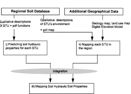
The general procedure used for mapping soil hy-draulic properties from qualitative descriptions of STUs of a small scale soil map is illustrated in Fig. 3. This approach includes three steps which are
Fig. 3. A general procedure for mapping soil hydraulic property from a regional soil database.
summarised below. More details can be found in Martin-Clouaire et al. (2000) and Cazemier (1999).
The first step (Fig. 3) consists in predicting the soil hydraulic properties of interest for each STU. This amounts to solving a system of equalities and inequal-ities as the following which estimates the available water capacity (awc).
w10=31.2−0.185∗sand+0.0675∗clay−7.63∗bulk density+Ierr1 w1500=39.9−0.094∗silt−0.204∗sand−12.3∗bulk density+Ierr2
awc=(w10−w1500)∗bulk density∗depth∗ 100
−stone
100
clay+silt+sand=100
w10> w1500
w10=4.66+0.914∗w1500+Ierr3
(1)
The first two equations are pedotransfer functions pro-viding an estimate of the water retention properties to determine awc. The third equation is the awc formula (Baize and Jabiol, 1995). The last three mathemati-cal expressions are constraints linking the variables of the first three equations. These relations express gen-eral physical rules or statistical knowledge from soil databases.
In the example shown, the variables clay, silt, sand, bulk density, depth and stone are imprecisely known and have values given by possibility distributions (see Section 2.1) representing fuzzy intervals. The error terms Ierr1, Ierr2 and Ierr3 are initially distributions of
regression residuals which are traduced into fuzzy in-tervals (Martin-Clouaire et al., 2000) for being com-patible with the other variables. The computation of
the fuzzy value of the awc is therefore an arithmetic calculus over non-independent fuzzy quantities which can be formulated as a fuzzy constraint satisfaction problem (CSP) (Dubois et al., 1993) without requir-ing any simplification hypothesis. In order to solve it efficiently, the constraint solver CON’FLEX (Reiller and Vardon, 1996) was used.
The second step of the spatial procedure is the map-ping of the STUs (Fig. 3). This involves examining each location in turn to find out the STUs that might be present on the basis of the environmental charac-teristics of the STUs and of the site. The estimation of the possibility that a particular STU is present at a particular site is done in two operations
• A fuzzy pattern matching (Badia and Martin Clouaire, 1989) for calculating for each environ-mental attribute the compatibility between the set of values characterising the STU as given by its qualitative description (Fig. 1) and the value taken by this attribute at the considered site as provided by the environment maps (geology map, DTM,. . .) included in the regional database. The matching may be partial due to the fact that the set may be
fuzzy and the retrieved value may be fuzzy too (Cazemier, 1999).
• A conjunctive combination (Dubois and Prade, 1988) which summarises the possibility values ob-tained for each individual attribute into a single possibility degree.
2.3. Estimating crop yields over the region
Once the techniques presented above are applied, estimation of crop yields over the region can be done, using the possibility distribution of soil parameters and climate parameters as inputs in a crop model.
The selection of the crop model is important. Obv-iously, it must be simple enough for being applica-ble over vast areas. However, a simple model has also its limitations in spatial applications (Leenhardt et al., 1995). A simple model generally neglects a lot of physical processes that limits its application to areas and topics in which these processes play a minor role. Furthermore, the cost reduction involved by limiting the measured physical parameters of complex models is often counteracted by the need of more local ex-perimental data for calibrating the global parameters considered in simple models.
A hybrid modelling approach containing two steps was applied in this study (Wassenaar et al., 1999): (1) running a mechanistic crop model over a set of soil–climate situations including the soil and climate variability of the studied region and (2) deriving a set of simple agrotransfer functions — linear or logarith-mic expressions — by regression analysis from the dataset obtained in the previous step. These agrotrans-fer functions can be considered as a very simplified crop model that can be used over vast areas. The main advantage of this method is that it integrates a mecha-nistic crop model for representing accurately the phys-ical process involved with the necessity of handling a very simple crop yield estimate, because of the limited data availability cited before. However, these agro-transfer functions have a limited sphere of validity. First, they are specific to a particular output of the crop model, e.g. the average hard wheat yield calculated over the 1984–1991 period for a wheat–maize (Zea
mays L.) rotation. Second, their spatial validity must
clearly be defined as demonstrated for similar mod-els like pedotransfer functions (Bastet et al., 1997). In the technique presented here, a reasoned sampling of soil–climate situations (Wassenaar et al., 1999) was necessary for obtaining an effective validity of the agrotransfer functions over the whole region.
The use of fuzzy estimates of soil parameter in the agrotransfer functions and the systematic presence of associated error terms expressed as fuzzy subsets leads to a fuzzy estimate of crop yield. This fuzzy estimate
of crop yield can be determined by arithmetic calculus with fuzzy quantities (Dubois and Prade, 1988). The use of CSP technique as the one involved for calculat-ing awc was not required here since no statistical rela-tions between agrotransfer funcrela-tions parameters were considered.
2.4. Mapping fuzzy estimates of crop yields
Mapping of crop yields over the region is of major concern for further decision making. A possibility distribution is a very complex information which cannot be summarised by a single value attached to a pixel. The proposed solution, as suggested by Hootsmans (1996) was two-fold: extracting synthetic indicators from the possibility distributions and using an interactive display environment.
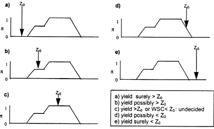
The synthetic indicators were derived in view to an-swer the following practical question: ‘Is the predicted wheat yield higher or lower than the given threshold value Z0?’ This type of question occurs frequently
since decision makers are very often interested in the position of this value relatively to a meaningful threshold value (e.g. the lowest value for economical viable cultivation of a specific crop). Fig. 4 illustrates how the results for each situation can be interpreted. Given a possibility distribution expressing the esti-mated crop yield at a point x (Mg ha−1), the value
of Z0 in relation to the distribution results in one
of five possible modalities, i.e. certainly above the threshold; possibly above the threshold; certainly be-low the threshold; possibly bebe-low the threshold; and undecided. The modality certainly above the
thresh-Fig. 4. Interpretation of possibility distributions of yield values (p) in order to map yield predictions. Z0 is a user-fixed threshold of
old means that the smallest value of the support of
the possibility distribution representing the hydro-logic property at point x is above the threshold. The modality possibly above the threshold means that the smallest value of the core of the possibility distribu-tion is above the threshold. The next two modalities were defined similarly. Undecided was used when the threshold falls within the core of the distribution (the true value can be above or below the threshold).
A Graphic User Interface for Windows (written in Delphi 3 (BorlandTM) using MapObjectsTM(ESRITM) was build for exploring interactively different values of the threshold Z0.
3. Application to the mapping of wheat yields over the Hérault-Libron-Orb valleys
3.1. The IMPEL project and the objective
The spatial procedure presented above was applied to the Hérault-Libron-Orb valleys (south of France) within the framework of the EC funded research project IMPEL (Integrated Model to Predict European Land use) (Rounsevell et al., 1998). This project aims at integrating physical and socio-economic models to evaluate the impact of climate change on Euro-pean land use systems at the regional scale. IMPEL is spatially distributed, based on a multidisciplinary, modular approach, and comprises
• a climate module to downscale baseline climate data (gridded to 0.5◦latitudinal/longitudinal) and Global Climate Model Experiment datasets (IPCC, 1995), using a stochastic weather generator,
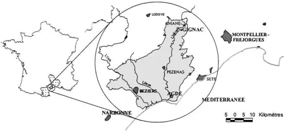
Fig. 5. Location of the study area in the Languedoc-Roussillon region, (Wassenaar et al., 1999).
• a soil and crop module to evaluate the soil water balance and crop yields for a wide range of Euro-pean crops,
• a land degradation module to evaluate the impact of soil erosion and changes in soil quality on crop productivity at the scale of soil map units and
• a socio-economic module to evaluate optimal land use allocation and management requirements at the scale of individual farms.
Application of the spatial procedure dealt only with the second module of the IMPEL model, i.e. the soil and crop model Euro-Access 2 (AgroClimatic Change and European Soil Suitability) developed earlier (Love-land et al., 1994). Spatial procedure was applied to the mapping of actual and expected crop yields over the demonstration region by coupling Euro-Access 2 with a set of soil and climate data, which were considered as easily available in almost all EC regions
• a 1:250,000 soil-landscape map of the region with a geo-referenced soil database in which STUs were described qualitatively as presented in Fig. 1,
• a limited set (<100) of profiles with soil descrip-tions and measurements of soil properties (texture, calcium content, organic matter content, bulk den-sity, water retention curve),
• pedotransfer functions providing hydraulic soil properties,
• maps of soil forming factors as relief (DEM), geo-logy or land-use over the studied region.
3.2. The region
1200 km2. The region exhibits typical northern Mediterranean climate characteristics, i.e. a substan-tial average annual rainfall (on average 700 mm per year), a high within-year rainfall variability with rain-fall peaks in autumn and spring and strong droughts in summer, high between-year rainfall variability, frequent and violent rainstorms and a large potential evapotranspiration (PET) (on average 1000 mm per year) due to the high average temperature and radia-tion and frequent and strong winds. The temperature exhibits only small variations across the studied re-gion (annual minimal temperature ranging from 8.7 to 10.1◦C, annual maximal temperature from 19.1 to 19.6◦C). Conversely, the weather stations within the region reveal a strong within-region-variability regarding rainfall (570–810 mm), which demonstrates a clear south–north gradient. PET measurements are only available from two weather stations, Narbonne and Montpellier-Fréjorgues which are situated at ei-ther side of the region (Fig. 5). The difference in an-nual average PET registered at both weather stations does not exceed 6%.
The regional soil pattern is extremely complex mainly due to the large geological variations. The ba-sic substratum is an heterogeneous Miocene marine sediment on which either Lithic Leptosols, Calcaric Regosols or Calcaric Cambisols (FAO-UNESCO, 1981) have formed. This substratum is partially overlain by Pleistocene alluvial deposits. These de-posits have produced stony soils ranging from Cal-caric to Chromic Luvisols. The most recent alluvial (Holocene) deposits contain Calcaric Fluvisols. Lo-cal volcanic activity and recent colluvial phenom-ena have contributed to the soil heterogeneity. The soil-landscape map of the studied region at 1:250,000 (Bornand et al., 1994) defines 36 soil-landscape units including 96 STUs in total.
3.3. Mapping hard wheat yields over the region
3.3.1. Deriving agrotransfer functions from a set of typical soil–climate situations
A limited number of simulation sites were selected in order to take into account the soil and climate vari-ability of the region (Wassenaar et al., 1999). Sixty-three soil profiles located within or at the vicin-ity of the study region were extracted from the Languedoc-Roussillon soil database (Bornand et al.,
1994) providing each of them the required input data for the Euro-Access model. The total set of profiles represented the range of soil types that occur in the region in terms of their hydraulic behaviour (Bornand et al., 1992; Bonfils, 1993).
Climate variability of the region was considered through a set of theoretical weather stations defined by assembling daily input data from available stations located within and near the study region. As stated in the previous section, temperature and PET exhibit only slight variations throughout the region, which allows the use of a unique data set of daily parameters, i.e. the one of the Montpellier-Fréjorgues weather station. Three weather stations, Béziers, Pézenas and Aniane, were selected to represent the south–north gradient as-sociated with change in elevation as this is the only noticeable climatic trend affecting the region.
The 63 soil profiles were combined with the three selected weather stations to obtain 189 theoretical soil–climate situations representing the range of soil– climate spatial variations observed within the region. The simulations were made using the crop model Euro-Access 2. A detailed description of the model and of the calibration protocol is provided in Wasse-naar et al. (1999).
Fig. 6 presents an example of agrotransfer func-tions obtained from the set of simulafunc-tions. The three presented agrotransfer functions estimate the average hard wheat yield for a wheat–wheat rotation for the period 1984–1991 as a function of awc for the three typical climate conditions of the studied region.
3.3.2. Estimating possibility distributions of available water capacity over the region
Fig. 6. Estimations of mean hard wheat yield over the period 1984-1991 for three representative climate situations (B´eziers, Aniane, P´ezenas), as a function of the soil awc. Correlation coefficients of curves fitted to the data are shown on the graph (Wassenaar et al., 1999).
distributions were defined according to the maximum admitted errors (Table 1). The qualitative descriptions of STUs do not include any information about the bulk density of the soil. Consequently, a unique pos-sibility distribution was defined for the region from a set of soil bulk density measurements. The core and the support of this distribution are given by the intervals (1.35, 1.60) and (1.15, 1.85), respectively.
Second, awc was mapped over the region follow-ing the scheme presented in Fig. 3. Available water capacities of the 96 STUs were determined accord-ing to Section 2.2. The points of the water retention curve involved in expressing awc were estimated by pedotransfer functions derived from dataset containing 372 measurements of hydraulic properties of soil hori-zons located in the Languedoc-Roussillon (Bastet et al., 1997). Different pedotransfer functions were cal-culated for four classes of substratum to increase the
Table 1
The maximum errors used for defining supports of possibility distributions
Variable Maximum error
Clay, silt, sand 100 g kg−1
Depth 10 cm
Stoniness 100 g kg−1
Organic matter content 10 g kg−1(lower classes)
50 g kg−1(upper classes)
Slope gradient 2 cm m−1(lower classes)
5 cm m−1(upper classes)
precision of estimations. A similar technique was ap-plied to determine the relation between the two points of the retention curve (last equation of system (1)). For each of these statistical relations, the error term was converted into possibility distributions. As stated in Section 2.2.1, the CSP solver CON’FLEX was used for calculating the final possibility distribution of awc per STU.
The presence of STUs was determined in terms of possibility at each node of a 100 m×100 m grid cov-ering the region according to Section 2.2. Additional geographical information involved in this step was as follows: (1) a slope gradient map derived from digi-tal elevation model at scale 1:25,000; (2) a 1:50,000 geological map and (3) a land use map derived from the 1:25,000 topographical map. The error terms as-sociated with (1) and the positional uncertainty of the boundaries of the map units of (2) and (3) were determined statistically by comparing with more pre-cise information which was available in some limited areas in the region like air-photograph-derived DEM, detailed soil maps (Cazemier, 1999). The possibil-ity theory algorithms required for calculating the possibility of presence of STUs (Section 2.2) were implemented in the macro language of Arc/InfoTM.
3.3.3. Applying agrotransfer functions with fuzzy estimates of available water capacity
The application of the agrotransfer functions amounts to a fuzzy calculus as presented in Section 2.3. Prior to this, each node of the grid covering the region was allocated to one of the three considered typical climate situations in view to select the adequate agrotransfer function. This was done by a nearest-neighbour algorithm. All these operations were per-formed within the GIS Arc/InfoTM.
3.4. Results and discussion
The evaluation of the estimates of awc by the pro-posed spatial procedure addressed two questions: (1) do the estimates match reality?, and (2) are they in-formative?
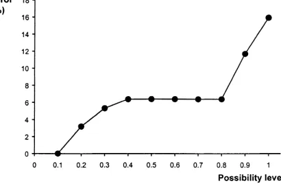
To answer the first question, a validation set of 111 sites with measured Euro-Access 2 soil inputs was considered in the study region. At each site, a mean annual wheat yield for the period 1984–1991 was cal-culated by an Euro-Access 2 simulation. To use these validation data for evaluating the spatial procedure, the estimated possibility distributions of wheat yield were first traduced into a set of crisp prediction inter-vals each defined by the two values of yield having a given possibility level (Fig. 7). The prediction inter-vals were then evaluated at each site by determining whether they include or not the calculated yields. Finally prediction errors were defined for each pos-sibility level by calculating over the set of validation sites the percentage of wrong predictions provided by intervals defined at the considered possibility level.
Fig. 8 shows the prediction errors calculated from the different levels of possibility. It reveals that the
Fig. 7. The definition of prediction intervals (black arrows) for possibility levels 0.1, 0.5 and 1 from estimated possibility distri-bution of yields (grey line).
Fig. 8. Prediction errors of yield estimates according to possibility levels p at which are defined prediction intervals.
proposed spatial procedure provided very reliable estimates since the error was never higher than 12% (possibility level=1). For possibility levels lower than 0.8, the predicted points were all included in the prediction intervals.
To determine whether the predictions are infor-mative or not, the widths of the prediction intervals derived from the estimated possibility distributions calculated over the whole region were considered. The larger the interval is, the less informative the pre-diction. For example, predicting that wheat yield is in the interval 3.5–4.8 Mg ha−1, is more informative
than predicting yield in the interval 1.5–4.8 Mg ha−1.
Fig. 9 illustrates the width of the predicted inter-vals over the region. The mean width (the black dots)
Fig. 10. Proportions of areas with the different possible answers given by the spatialisation procedure for different user-fixed thresh-olds of yield.
ranged between 4.4 and 8 Mg ha−1. These values
de-note that the predictions were, in general, not very informative. The width of intervals for the lower lev-els of possibility (<0.6), was even larger than the total range of variations observed in the validation dataset (0.67–7.42 Mg ha−1). However, as shown by the
con-fidence intervals of the highest level of possibility (the grey vertical bars), the interval width exhibited a substantial variation around the mean, suggesting that more informative predictions could be found for limited areas in the study region.
In order to evaluate this, Fig. 10 presents the evo-lution of the areas covered by each decision unit de-scribed in Section 2.4 with respect to a yield threshold value. This figure demonstrates clearly that the ability to provide an informative result depends strongly on the query, i.e. of the considered threshold value. When the threshold ranged between 2–5.5 Mg ha−1, the
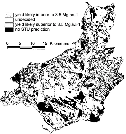
pro-portion of areas for which no decision can be made (undecided) predominated. However, an informative answer could be given for most locations when ex-treme threshold values were considered. As expected, the proportion of undoubted answers remained low, whatever the threshold value considered. On the other hand, for all threshold values, it was possible to identify small but significant areas that have extreme behaviour with regard to the question posed. For example, the spatial procedure identified within the region 127 km2 where hard wheat yields were likely to be greater than 3.5 Mg ha−1, and 21 km2 where
hard wheat yields were likely to be less than this threshold value. The corresponding map is provided in Fig. 11.
Fig. 11. An example of hard wheat yield map over the region for the threshold 3.5 t ha−1.
4. Conclusions
There is a need to develop spatial procedures for mapping crop yield over vast areas where quantitative soil information required by crop models is system-atically scarce. In these situations, the use of the available qualitative soil information and the prop-agation of the various uncertainties associated with this kind of information are of paramount importance. Based on this perspective, this study proposed a spa-tial procedure based on possibility theory and CSP algorithms. Crop modelling results were summarised by agrotransfer functions which were applied for a given situation and a given query. The procedure was tested in the Hérault-Orb-Libron valleys region.
classical mapping was to identify the queries and the areas for which no information can be reasonably de-livered. However, the validation results suggested that more informative estimates could be obtained with the same source data by modifying the parametrisation of the possibility distributions derived from the soil database. In the current situation, the range of really useful possibility levels at which estimates are deliv-ered was very small since below possibility level 0.6, the estimates do not bring any information about the possible values of yields. Since the prediction errors were shown to be very low, higher risk can be accepted when interpreting the input soil data — i.e. to reduce the width of both core and support of the possibility distributions — which can lead to more informative estimates. This would be easier if a better knowledge of the uncertainty associated with the soil data could be collected in regional databases.
In any case, this case study demonstrated that a significant effort must be made for increasing the pre-cision of yield estimates over vast areas. Several pos-sible improvements of the existing soil databases can be envisaged such as extending the range of system-atic soil characterisation (e.g. bulk density), deriving more precise pedotransfer functions, providing more accurate descriptions of STUs (e.g. by means of range of values by soil horizons), and enlarging the mapping scale in view to locate the STU. To define priorities among all these possible improvements requires a cost-utility analysis which should take into account the variety of situations of a given region. The pro-cedure presented in this paper could be useful in this perspective.
Acknowledgements
The research reported in this article was under-taken within the IMPEL project, and funded by the European Commission under the Climate and En-vironment Programme of Framework IV (Contract no. ENV4-CT95-0114). The authors thank Dr. Mark Rounsevell (University of Catholique de Louvain) for leading the IMPEL project. The authors also thank J.P. Barthès, Dr. M. Bornand and P. Falipou for pro-viding the soil data used in the study and Alfred Stein for his useful comments and corrections on an earlier version of the manuscript.
References
Akinremi, O.O., McGinn, S.M., Howard, A.E., 1997. Regional simulation of fall and spring soil moisture in Alberta. Can. J. Soil Sci. 77, 431–442.
Badia, J., Martin Clouaire, R., 1989. Choice under imprecision: a simple possibility-theory-based technique illustrated with a problem of weed identification. Comput. Electron. Agric. 4, 103–120.
Baize, D., Jabiol, B., 1995. Guide pour la description des sols, INRA, Versailles.
Bastet, G., Bruand, A., Voltz, M., Bornand, M., Quétin, P., 1997. Performance of available pedotransfer function for predicting the water retention properties of French soils. In: Proceedings of the International Workshop on New Developments in Estimating the Hydraulic Properties of Unsaturated Soils, Riverside, CA, USA.
Bonfils, P., 1993. Carte pédologique de France à 1/100 000. Feuille de Lodève, SESCPF INRA, Orléans.
Bornand, M., Barthès, J.P., Bonfils, P., 1992. Carte des pédopaysages du Languedoc Roussillon à l’ échelle du 1/250 000. Laboratoire de Science du Sol, Montpellier. Bornand, M., de Laroche, E., Legros, J.P., 1998. Soil water
balance of the vineyard of the Languedoc: a tool for rural area management. In: Proceedings of the XVIth World Congress of Soil Science, Montpellier, France.
Bornand, M., Legros, J.P., Rouzet, C., 1994. Les banques régionales de données-sols. Exemple du Languedoc-Roussillon. Etude et Gestion des Sols 1, 67–82.
Bouma, J., van Lanen, J.A.J., 1987. Transfert functions and threshold values: From soil characteristics to land qualities. In: Beek, K.J., Burrough, P.A., McCormack, D.E. (Eds.), Proceedings of the ISSS and SSSA International workshop on Quantified Land Evaluation, ITC no. 6, Washington DC, USA. Cazemier, D., 1999. Utilisation de l’information incertaine dérivée d’une base de données sols. Application à la cartographie des propriétés hydriques à l’échelle régionale. Thèse Doctorat, Ecole Nationale Supérieure Agronomique, Montpellier. Dubois, D., Prade, H., 1988. Possibility Theory: An Approach to
Computerized Processing of Uncertainty, Plenum Press, New York.
Dubois, D., Fargier, H., Prade, H., 1993. Propagation and satisfaction of fuzzy constraints. In: Yager, R., Zadeh, L. (Eds.), Fuzzy Sets, Neural Network and Soft Computing. Kluwer Academic Publishers, Dordrecht, pp. 166–187.
Dumanski, J., Pettapierce, W.W., Acton, D.F., Claude, P.P., 1993. Application of agro-ecological concepts and hierarchy theory in the design of databases for spatial and temporal characterisation of land and soil. Geoderma 60, 343–358.
Fabre, J.C., 1998. Interface d’utilisation d’un résolveur de contraintes floues à l’usage d’un Agronome (CAPRISI), USTL, CNIAM, Montpellier.
FAO-UNESCO, 1981. Soil Map of the World at 1: 5,000,000. Food and Agriculture Organisation, Rome.
IPCC, 1995. Climate Change 1995: The Science of Climate Change. Cambridge University Press, Cambridge.
King, D., Daroussin, J., Tavernier, R., 1994. Development of a soil geographic database from the soil map of the European communities. Catena 21, 37–56.
Le Bas, C., King, D., Daroussin, J., Nicoullaud, B., Ngongo, M., 1998. Impact of errors in the assessment of agronomic constraints to crop production at a European scale. In: Proceedings of the XVIth World Congress of Soil Science, Montpellier, France.
Leenhardt, D., Voltz, M., Rambal, S., 1995. Survey of several agroclimatic soil water balance models with reference to their spatial application. Eur. J. Agron. 4, 1–14.
Loveland, P.J., Legros, J.P., Rounsevell, M.D.A., de la Rosa, D., Armstrong, A., 1994. A spatially distributed soil agroclimatic and soil hydrological model to predict the effects of climate change within the European community. In: Proceedings of the XV World Congress of Soil Science, Vol. 6a, Commission V, Acapulco, Mexico, pp. 83–100.
Martin-Clouaire, R., Cazemier, D., Lagacherie, P., 2000. Representing and processing uncertain soil information for mapping hydrological soil properties. Computer & Electronics in Agriculture, in press.
Oldeman, L.R., van Engelen, V.W.P., 1993. A world soils and terrain digital database (SOTER) — an improved assessment of land resources. Geoderma 60, 309–325.
Reiller, J.P., Vardon, F., 1996. CON’FLEX version 1.0. Manuel de l’utilisateur. Laboratoire de Biométrie et d’inte-lligence Artificielle INRA Toulouse, http://www-bia.inra.fr, Toulouse.
Rounsevell, M., Armstrong, A., Audsley, E., Brown, O., Evans, S., Gylling, M., Lagacherie, P., Margaris, N., Mayr, T., de la Rosa, D., Rosato, P., Simota, C., 1998. The IMPEL project: integrating biophysical and socio-economic models to study land use change in Europe. In: Proceedings of the XVIth World Congress of Soil Science, Montpellier, France.
Smaling, E.M.A., Fresco, L.O., 1993. A decision support model for monitoring nutrient balances under agricultural land use (nutmon). Geoderma 60, 235–256.
Staff, S.S., 1993. Soil Survey Manual, USDA.
Wassenaar, T., Lagacherie, P., Legros, J.P., Rounsevell, M.D.A., 1999. Modelling wheat yield responses to soil and climate variability at the regional scale. Clim. Res. 11, 209–220. Zadeh, L., 1978. Fuzzy sets as a basis for a theory of possibility.