Data assimilation techniques and modelling uncertainty in geosciences
Mehdi Darvishi a, *, Gholamreza Ahmadib
a PhD Candidate in Remote Sensing, Department of Remote Sensing and GIS, Geography Faculty, TehranUniversity, Tehran, Iran [email protected]
b PhD Candidate in meteorology, Department of Geography, Science and Research Branch, Islamic Azad University, Tehran, Iran [email protected]
KEY WORDS: Data assimilation (DA), Uncertainty, 4D-VAR, Minimization, Cost function, Kalman filter
ABSTRACT:
"You cannot step into the same river twice"1. Perhaps this ancient quote is the best phrase to describe the dynamic nature of the earth system. If we regard the earth as a several mixed systems, we want to know the state of the system at any time. The state could be time-evolving, complex (such as atmosphere) or simple and finding the current state requires complete knowledge of all aspects of the system. On one hand, the Measurements (in situ and satellite data) are often with errors and incomplete. On the other hand, the modelling cannot be exact; therefore, the optimal combination of the measurements with the model information is the best choice to estimate the true state of the system. Data assimilation (DA) methods are powerful tools to combine observations and a numerical model. Actually, DA is an interaction between uncertainty analysis, physical modelling and mathematical algorithms. DA improves knowledge of the past, present or future system states. DA provides a forecast the state of complex systems and better scientific understanding of calibration, validation, data errors and their probability distributions. Nowadays, the high performance and capabilities of DA have led to extensive use of it in different sciences such as meteorology, oceanography, hydrology and nuclear cores. In this paper, after a brief overview of the DA history and a comparison with conventional statistical methods, investigated the accuracy and computational efficiency of two main classical algorithms of DA involving stochastic DA (BLUE2 and Kalman filter) and variational DA (3D and4D-Var), then evaluated quantification and modelling of the errors. Finally, some of DA applications in geosciences and the challenges facing the DA are discussed.
*Corresponding author.
1Heracleitus, Trans. Basil. Phil. Soc. Miletus, cca.500 B.C. 2Best Linear Unbiased Estimator
1. MANUSCRIPT
1.1 Introduction
The first application that has motivated the growth of data assimilation is weather forecast, but nowadays its applications have been developed from weather forecast to engineering and geosciences applications. Increasing availability of acquired observations from satellite instruments and the role of propagating observational information in time (in addition to the spatial interpolation) are the reasons that lead us to necessity of having a synoptic view of the state of the system from asynoptic data. The difficulty is to use these data, which are sometimes conflicting, to find a best estimate of the state of the earth system which will be used for diverse applications. But we need to ensure that a time sequence of these estimated states is consistent with any known equations that govern the evolution of the system. The method to achieve this goal is known as data assimilation [Mathieu and O’Neill, 2008]. Data assimilation is a set of techniques thereby information from observations is optimally combined with model and it will estimate the state of an unknown system based on an imperfect model and a limited set of noisy observations. Over the past decades, numerous algorithms were developed by scientists. The summary of data
concerned with the estimation of initial conditions. By contrast, land surface dynamics are damped, and land surface assimilation is all about estimating errors in uncertain meteorological forcing (boundary) conditions and model parameterizations [Reichle, 2008] The roll of error modelling and error statistics uncertainty analysis play great role in forecasting and parameters estimation of complex systems state.
End of the 18th century Planet orbit computations by Gauss
Least square method by Legendre Beginning of the 20th century Concept of maximum likelyhood by Fisher
Mid of the 20th century Kalman filter for the APOLLO program Objective analysis of meteorological fields
End of the 20th century
3D-var data assimilation method for weather forecast model Gain of 20% forecast quality at Météo-France going to 4D-var
Table 1. A summary of data assimilation history
1.2 Definitions and basic concepts
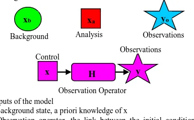
First, we must define the parameters and properties of the model and its relationship with observations. Variables are defined the following:
x: Inputs of the model
xb: Background state, a priori knowledge of x
H: Observation operator, the link between the initial condition and Observations: y=H(x)
y: Vector of modelled observations, i.e., the outputs of the model yo: Vector of observations (true measurements)
xa: Analysis model state
Figure 1. Variables and operators involving at DA
2. METHODS
2.1 Stochastic data assimilation
2.1.1 The best linear unbiased estimate (BLUE)
For estimation the true state xt of a system, by assuming some assumptions involving unbiased data, the observation operator is assumed linear and the uncertainties are given in the form of the covariance matrices R and Pb, we will have:
y Hxt , =0 , Pt b bT , R T Mentioned linear combination of the observation and the background terms gives the best estimation of true state:
x =a Ax +b Kyb
A and K are coefficients are characterized for the estimation optimal. By an unbiased estimate with minimum variance condition, we will reach to the estimation optimal, i.e.
a =0
, tr
Pa min imumWhen those conditions are satisfied that the following equations established:
A= -K K=P Hb T
HP Hb T+R
-1 (1) K is called the Kalman gain. The final form of the equation isxaxbK
y Hxb
Pa=
I KH P-
b (2)superscript is a time that pointing observation dates. We assume
to have the Following assumptions: 1- The initial state x t0and
the model errors ηkare gaussian-distributed with mean x0band covariance Qk respectively 2- Again, observation operators is
linear. Under these hypotheses, KF presented the estimate of the
statesxtk. KF is a sequential algorithm and divided into two
steps: analysis and forecast steps.
Analysis step: we know P x k y0:k-1
Pf values (a in subscript xak donates with the analysis):
estimation ofxtk+1by using dynamical model, it is provided the
Based on what mentioned above, KF is started with a forecast
state xfand error covariancePfthen the assimilation sequence
is done by KF equations. There are some important issues about implementation of KF algorithm that should be noticed. In following we will mention these implementation problems.
Dimensions Problem
The size of state covariance matrix is one of the implementation issues in KF algorithm, especially in oceanography or meteorology applications that models usually include millions or even tens of millions of variables. The common solution to this problem is rank reduction of the state covariance matrix by some mathematical methods such as Square-root decomposition.
Filter Divergence Problem
Filter divergence problem occurs when the input statistical data are mis-specifed. As a result, filtering system goes to underestimate of the error variances and it is caused some observations ignored by the system (due to the too much confidence is given in state estimation step).
Symmetric Covariance Matrix Problem
The matrix equation (6) yields a symmetric matrix, but we practically encounter with an asymmetric covariance matrix, Therefore the filter cannot work correctly. One way to solve this problem is to add additional step to reach the symmetric matrix or using the square root form of covariance matrix.
Nonlinear dynamics problem
Nonlinearity of model M (such as second-order equations in atmospheric and Oceanic models) and observation operator H (such as the radiance parameter at optical satellite observations) in KF causes two main problems: 1- nonlinearity damages gaussianity of statistics 2- Failure to define the transposed model. One way that we can adapt the nonlinear models and observations with KF algorithm is to use the Extended Kalman Filter (EKF). The EKF uses M and H (tangent linear of M and H) in equations of analysis and forecast steps. In the next section, we will introduce an efficient method called variational data assimilation for solving the nonlinear dynamics problem.
2.2 Variational Data Assimilation
If the observation operator is found to be linear in cost function, it leads to the Best Linear Unbiased Estimation (BLUE) method. But at the time evolution models that measurements spread on a time interval, the cost function uses the computation of adjoint model for minimization. Most of the data assimilation algorithms often result in a cost function that must be minimized (a typical cost function shown in figure 2). This cost function has quadratic forms and including observation and background covariance matrices. Equation 7 shows a typical form of the cost function. Regarding a large number of parameters acquired from satellite observations with high spatial and temporal scales, solving the high-dimensional and
nonlinearity problems of observations are inevitable. The goal is finding the minimum x of a quadratic cost function in equation 7.
J( )=
1/2║
-
║
2B
+
1/2║
-
║
2RFigure 2. A simple example of distances minimization (weather forecast and estimation application) [Thual, 2013].
b
T T
x x - xb x - xb y - H x y - H x
J J
1 1
J B R (7)
B: covariance matrix of the background errors R: covariance matrix of observation errors
Solving the problem of minimization needs efficient and advanced numerical methods to minimize J. we are searching for a state trajectory x that is satisfying the background error statisticsJb, with the least distance to the observation. Since J is quadratic and strictly convex, therefore definitely exists at least a unique minimum or there maybe some local minima. The goal is to find this minimum or minima. In the following, some of the most important of minimization algorithms will be pointed. For more information and details you can see [Bishop, 1995], [Saporta, 2005] and [Tarantola, 2005].
2.2.1 Minimization Algorithms
2.2.2 Newton algorithm
As we know from mathematics, a minimum of the function J is, the gradientJ, equal to zero. Newton Algorithm takes an iterative approach to reach the minimum of the J:
k k k
x x .J
k
1 1
H (8)
k
H is the Hessian matrix (square matrix of second-order
partial derivatives of a function). Because of following reasons this algorithms could become unstable: a) assessment of
k
H and also obtaining the matrix inverse of Hkneed computations and it is possible the matrix size of second terms of equation 6 become larger than a size that can be validated.
2.2.3 Quasi-Newton algorithm
Quasi-Newton algorithm creates an approximation to the inverse Hessian over iterative steps, contrary to Newton algorithm that initially computed Hessian matrix directly and then investigating its inverse. Despite the algorithmic complexity, it provides a good convergence speed rather than Newton algorithm.
2.2.4 3D-VAR and 4D-VAR analysis
One of the most important variational data assimilation, that it is based on the 3D-VAR algorithm, is 4D-VAR algorithm. We seek for an approximate solution to the equivalent minimization problem with J. With descent algorithm, we can reach the minimum value, by gradient of the cost function:
x 2 1
x xb 2H -1
y x
T
J B R H (9)
The minimization process can be stopped by specific number of iterations or by a predefined amount of incremental norm of the gradient J
x during the minimization. The geometry of theprocess is shown in Figure 4.
Figure 4. Minimization of cost function and its gradient. The shape of J
x is a paraboloid with the minimum at the optimalanalysis xa. Figure from [Bouttier and Courtier, 1999].
Although 3D-VAR dose not need to compute the gain K in equation (1), it requires designing a model for B. 3D-VAR gives us a global analysis that can be applied to any observation, especially in the case of nonlinear observations.
When the observations are distributed in time, we use the simple generalization of 3D-VAR that called 4D-VAR. There is no considerable difference between 3D-VAR and 4D-VAR, the equations are the same. In figure 5 we can see the differences and similarities. The main difference related to the observations at different times in the definition of theJ
x :
x
y x
R y x
x x x xT n
-1 b -1 b
i i i i i i i
i 0
J H H B (10)
Index i denotes the observation at any time.
Figure 5. The comparison between 3D-VAR and 4D-VAR. Figure from [Holm, 2003]
4D-VAR behaves like the integration of an adjoint model backward in time, it try to find the initial condition for the forecast that has the best fit for the observations. In this algorithm if M and H are nonlinear, 4D-VAR uses adjoint methods for computation of gradient, because the result of the gradient remains exact. 4D-VAR algorithm provides an efficient tool for numerical forecasting. The graphical function of 4D-VAR process is provided in figure 6.
Figure 6. Example of 4D-VAR assimilation in a numerical forecasting system. Every 6 hours a 4DVAR is performed to assimilate the most recent observations, using a segment of the previous forecast as background. This updates the initial model trajectory for the subsequent forecast. Figure from [Bouttier and Courtier, 1999].
2.3 Error quantification and modelling in data assimilation
Since to get the best estimation all data must be combined in statistical methods, therefore having a reliable and accurate error statistics is necessary. As we know, models in the real world are chaotic and nonlinear; therefore errors exist in background, observation and analysis parts of DA. For statistical analysis of error, we initially assume probability density function (pdf) for errors. According to the definitions of the figure 1:
x x b b t
Error covariance is a appreciate tool for analyzing the error. The errors are considered based on the two statistical parameters (i.e. biases and covariance matrix). Errors are functions of our a priori knowledge of the errors, background and observations. In general, for computing the error statistics is to assume that the errors are uniform over the interval and stationary over a period of time (called ergodicity assumption). For the suitable quality of the analysis, we need a proper statistics of background and observation error covariances. The necessary parameters are correlations and variances. The observation error variances, we must not permit to the observation biases contribute to the observation error variances, because it creates biases in the analysis increments. Therefore, after determining the observation biases, it must be removed from observation and background. The observation error correlations, they are often zero (an assumption). This assumption about observations that acquired from different instruments is correct, but about the observations acquired from the same platform such as satellite observations and radiosonde are not the proper assumption. The estimation of observation error correlations is not easy task and often causes problems in the quality of control algorithms and numerical analyses. The background error variances estimate in forecast step and in KF algorithm they estimate by tangent-linear model. Among the mentioned statistical parameters of errors in the first part of this section, Background error correlations is placed on the specific site, because following reasons: 1) when the data in an area are Sporadic, the form of the analysis increment is specified by the covariance structures and correlations of B shows the spatial distribution of data from the observations, this fact often called Information spreading, 2) since the degrees of freedom in a model are more than in reality, the balance properties (refer to the stable properties of a system, for example, hydrostatic properties of atmosphere) impose some unwanted and annoying limitations on the analysis step. Using covariance matrix B help to better error analysis, for more details see [Bouttier and Courtier, 1999], 3) when the data in an area are dense, correlations in B is the best index for discrete observations the amount of smoothing of the observed data (called information smoothing). Since the errors can only be estimated by statistical fashion and they cannot be seen directly, the most suitable way to consider the errors is to evaluate
yH
xb
. Also we can use some empirical methods(forecast-based) such as NMC algorithm or adjoint sensitivity.
3. Applications
3.1 Applications of data assimilation in geosciences
Atmosphere
The applied use of variational assimilation techniques returns to the mid-1980s. At first, thses methods were used to assimilating radiosonde observations over a 24-h period in northern hemisphere. The researchers founded that these techniques can reconstruct all structures of the flow resolvable by the model to an accuracy of about 30 m for geopotential heights
and8ms1for wind vectors (Courtier and Talagrand[1987] and Talagrand and Courtier[1987]. Also assimilation techniques have a wide range use in atmospheric chemistry field and especially assimilating the measurements of global circulation
models and chemistry-transport model. One of the most significant uses of assimilation techniques is to understanding of the global carbon cycle. For instance, we can point to estimating atmospheric CO2 from advanced infrared satellite radiances within an operational (4-D VAR) data assimilation system (Engelen and McNally [2005]). In assimilation data, 3D atmospheric indices such as humidity, temperature, winds, pressure can be considered as Control vectors x and Satellite data or In-situ data can be assumed as Observations vector y. Weather forecast is the most significant application of data assimilation in meteorological models.
oceanography
In oceanography studies, reconstructing, monitoring and forecasting the state of the ocean are pillars of this science. Data assimilation gives us initial conditions for monthly and seasonal forecasts. Although ocean observations are less than atmospheric observations, DA can decrease the large uncertainty (due to the forcing fluxes). As mentioned in the previous section, in the case of oceanography, currents, temperature and salinity observations (3D) and altimetry (2D) can be considered as Control vectors x and so on. A number of DA has been developed for linear ocean models and ocean circulation models [Fukomori and Malanotte-Rizzoli, 1995- Ngodock et al., 2000]. One of the main problems in ocean modelling process is bias and DA is an efficient way of controlling model bias. Also DA provides ocean reanalysis for instance, SODA3 ( using sequential OI technique) and GECCO4 (using variational DA).
4. Conclusion
Our ability to accurately characterize large-scale variations in geosciences applications is severely confined by process uncertainty (error) and imperfect models. Assimilation data as an analysis that combines time-distributed observations and a dynamic model is a technique to overcome these restrictions. In real world when we face nonlinear chaotic systems that involving high flow dependent variability of error dynamics such as Atmosphere and Ocean, therefore having accurate and proper description of the error entering the estimation is necessary. Nonlinearity is a problem that spoils Gaussianity, it could be related to the observation operator H the model and or initial guess B. Variational and ensemble schemes are two main solutions for solving that problem. Each of them has drawbacks and abilities. For example, some drawbacks of variational method can be noted: 1) Lack of being Non-quadratic J(x) in 4D-VAR, 2) Having several Multiple Minima in cost function. Of course, there are ways to overcome mentioned problems (for example, using incremental 4D-VAR for problems 1and 2). The drawbacks of ensemble methods can include: 1) Sampling error, 2) observations must be used at analysis time, 3) Gaussian distribution assumption ofPf. Again, there are solutions for solving or alleviating the problems such as, using covariance localization or additive inflation for problem (1), using hybrid method (several ensemble schemes) for problem (2), and using Particle Filters for problem (3). Despite the computational and statistical abilities of DA algorithms, there are still big challenges and difficulties for data assimilation techniques involving:
Background Error Covariance Modelling
reduction of systematic errors in the model and observation
Processing of data to approximate Gaussianity
Model errors and Non-Linearities
Data assimilation techniques have traveled long path so far, from meteorology applications in the past to the engineering applications in the current era, this vicissitudes path still continues.
REFERENCES
Bishop, C. M., 1995. Neural Networks for Pattern Recognition. Oxford University Press, 482 pp.
Bouttier, F., and Courtier, p., 1999, Data assimilation concepts and methods. Training Course notes of ECMWF, 59 pp.
Courtier, P. 1997, Variational methods, J. Meteorol. Soc. Jpn., 75, 211–218.
Courtier, P., and Talagrand, O., 1987. Variational assimilation of meteorological observations with the adjoint vorticity equation. II: numerical results theory, Q. J. R. Meteorol. Soc., 113, pp. 1329–1347.
Daley, R., 1993. Atmospheric Data Analysis. Cambridge University Press.
Engelen, R. J., and McNally A. P., 2005. Estimating atmospheric CO2 from advanced infrared satellite radiances within an operational four-dimensional variational (4D-Var) data assimilation system: Results and validation, J. Geophys. Res., 110, D18305.
Fukumori, I., and Malanotte-Rizzoli, P., 1995. An approximative Kalman Filter for ocean data assimilation: An example with an idealized Gulf stream model, J. Geophys. Res., 100, 6777–6793.
Gelb, A., 1974. Applied Optimal Estimation. MIT Press, Cambridge, Mass, 374 pp.
Hòlm, E. V., 2003. Lectures notes on assimilation. Training Course notes of ECMWF, 30 pp.
Lions, J.-L., 1971. Optimal Control of Systems Governed by Partial Differential Equations, 396 pp., Springer, Berlin.
Lorenz, E., Emmanuel, K., 1998. Optimal sites for supplementary weather observations: simulation with a small model. J. Atmos. Sci. 55, 399–414.
Mathieu, P.-P., and A. O’Neill, 2008. Data assimilation: From photon counts to Earth System forecasts, Remote Sens. Environ., 112, 1258–1267.
Ngodock, H. E., B. S. Chua, and Bennett A. F., 2000, Generalized inverse of a reduced gravity primitive equation model and tropical atmosphere-ocean data, Mon. Weather Rev., 128, 1757–1777.
Reichle, R. H., 2008. Advances in Water Resources., 31, pp. 1411–1418.
Saporta, A., 2005. Probability, Data Analysis and Statistics. Technip, Paris, 656 pp.
Thual, O., 2013. Introduction to Data Assimilation for Scientists and Engineers. Institut National Polytechnique de Toulouse), pp. 15-16.
Talagrand, O., and Courtier, P., 1987. Variational assimilation of meteorological observations with the adjoint vorticity equation. I: Theory, Q. J. R. Meteorol. Soc., 113, 1311–1328.
![Figure 3. Schematic shows a cost function and minimization process. Figure from [Bouttier and Courtier, 1999]](https://thumb-ap.123doks.com/thumbv2/123dok/3257560.1399406/3.595.331.514.488.643/figure-schematic-function-minimization-process-figure-bouttier-courtier.webp)
![Figure 5. The comparison between 3D-VAR and 4D-VAR. Figure from [Holm, 2003]](https://thumb-ap.123doks.com/thumbv2/123dok/3257560.1399406/4.595.95.254.521.653/figure-comparison-d-var-d-var-figure-holm.webp)
