LEARNING IMAGE DESCRIPTORS FOR MATCHING BASED ON HAAR FEATURES
L. Chen, F. Rottensteiner, C. Heipke
Institute of Photogrammetry and GeoInformation, Leibniz Universität Hannover, Germany - (chen, rottensteiner, heipke)@ipi.uni-hannover.de
Commission III, WG III/4
KEY WORDS: Image Descriptors, Descriptor Learning, Haar Features, AdaBoost, Image Matching, Pooling Configuration
ABSTRACT:
This paper presents a new and fast binary descriptor for image matching learned from Haar features. The training uses AdaBoost; the weak learner is built on response function for Haar features, instead of histogram-type features. The weak classifier is selected from a large weak feature pool. The selected features have different feature type, scale and position within the patch, having correspond threshold value for weak classifiers. Besides, to cope with the fact in real matching that dissimilar matches are encountered much more often than similar matches, cascaded classifiers are trained to motivate training algorithms see a large number of dissimilar patch pairs. The final trained output are binary value vectors, namely descriptors, with corresponding weight and perceptron threshold for a strong classifier in every stage. We present preliminary results which serve as a proof-of-concept of the work.
1. INTRODUCTION
Feature based image matching aims at finding homogeneous feature points from two or more images which potentially contain the same object or scene. Feature detection, description and matching among descriptors form the feature based local image matching framework. Matching algorithms should be robust to image transformations, while recalling as many matching points as possible and maintain as high an overall geometric accuracy as possible. Another important aspect is the speed of computation, where naturally faster means better when high recall and accuracy are guaranteed.
To cope with geometric and radiometric transformations, SIFT (Lowe, 2004) and SURF (Bay et al., 2008) apply a set of hand-crafted filters and aggregate or pool their responses within pre-defined regions of the image patch (Trzcinski et al., 2012). The extent, shape and location of these regions form the pooling configuration of the descriptors. Specifically, SIFT uses grid regions and aggregates by histogram of gradients in rectangular grid regions. In other descriptors such as SURF (Bay et al., 2008) and DAISY (Tola et al., 2010), the shapes of these pooling regions vary from grid to concentric circles around the centre of the patch.
Building a descriptor can be seen as a combination of the following building blocks (Brown et al., 2011a): 1) Gaussian smoothing; 2) non-linear transformation; 3) spatial pooling or embedding; 4) normalization. If we take matching image patch pairs as positive matches and non-matching patch pairs as negative matches, image matching can be converted to a two-class two-classification problem. For the input training patch pairs, the similarity measure based on every dimension of the descriptor is built. Fed with training data, the transformation, pooling or embedding that gets minimum loss can be found to build a new descriptor.Work in (Brown et al., 2011a, Trzcinski et al., 2012) has proved that blocks 2) and 3) can be learned and the learned descriptors can improve matching performance significantly. The parameters of these descriptors are trained and optimized on large training data set.
Cai et al., (2011) learn descriptors from the perspective of embedding. The Local Discriminant Projection (LDP) is presented in their work to reduce the dimensionality and improve the discriminability of local image descriptors. In the work of (Brown et al., 2011), non-linear transformation and pooling / embedding are added to the learning parts. However, predefined pooling shapes are used, similar to the SIFT rectangular grid and the GLOH (gradient location and orientation histogram) log-polar location grid. In GLOH, a SIFT descriptor is computed with three bins in radial direction and eight in angular direction. But its learning criterion, area under the receiver operating characteristic (ROC) curve, is not analytical and hard to optimize. Convex optimization (Simonyan et al., 2012) is used to learn optimal pooling configurations. Another idea is to use weak learners based on comparison or statistics, and use boosting to obtain the optimal pooling configuration and embedding simultaneously (Trzcinski et al., 2012).
In most of the current descriptor learning work, algorithms use the same amount of positive and negative training data, which is in contrast to the real situation in feature based matching: the number of dissimilar matches is much higher than the number of correct (similar) matches. In particular, without prior knowledge, every interest point patch should be matched to all interest point patches from another image. As true match pairs are rare, most of these matching hypotheses will be incorrect. Therefore, in a real matching scenario, a negative matching output appears much more often than a positive output. Perhaps more importantly: incorrect pairs will have a broader statistical distribution and more learning pairs are required to represent this distribution.
Inspired by the above points, multi-stage cascaded learning is used in our work. New negative training samples, which are non-separable in former stages, can be added in the next stage, and then the discrimination of the learned descriptor can improve as the number of stages increases. By training in this cascaded way, the learning algorithm can see large numbers of The International Archives of the Photogrammetry, Remote Sensing and Spatial Information Sciences, Volume XL-3, 2014
negative samples. More importantly, in the early stages descriptors are tuned to eliminate negative matching pairs reliably, a large number of wrong matches will be eliminated early and later stages only focus on promising candidate pairs. Therefore the matching can be speeded up.
On the other hand, different transformations in the non-linear transformation stage correspond to different kinds of weak features for learning. There are mainly two kinds of features: comparison-based and histogram-based features. Normally, comparison-based features lead to binary descriptors and histogram-based features lead to floating point descriptors. A point worth noting here is histogram-based features need more complex computation than comparison-based weak features. In our work, Haar features are used in combination with threshold perceptron. They can be computed efficiently using the concept of integral images and each dimension can be calculated using only a few basic operations like addition, subtraction and value accessing, thus the descriptor building computation speed can be boosted. Besides, the output descriptors are binary vectors, therefore the speed of similarity computation can benefit again from Hamming distance computations.
2. RELATED WORK
Descriptors are built on the patch surrounding a feature point. SIFT (Lowe, 2004) is the well-acknowledged breakthrough descriptor, in which grid pooling shapes are designed and gradient features in each pooling region are aggregated by histograms. Further works inherit this pooling and aggregation principle and introduce dimension reduction, like PCA-SIFT (Ke & Sukthankar, 2004), which lowers the descriptor from 128 dimensions to 36 dimensions by PCA, but applying PCA slows down the feature computation (Bay et al., 2008). An alternative extension, GLOH (Mikolajczyk et al., 2005), changes shapes of pooling from rectangular grid to log-polar grid, whereas DAISY (Tola et al., 2010) extends the pooling region to concentric circles. Another landmark work, SURF (Bay et al., 2008), mainly benefits from using integral images and approximation box filters for first-order, second-order and mixed partial derivatives. It finishes matching in a fraction of the time SIFT used while it achieves a performance comparable to SIFT.
Another important category, binary descriptors, are widely used to reduce memory requirements to boost the speed of similarity and matching computation. Local Binary Patterns were first used to build a descriptor in (Heikkilä et al., 2009). Each dimension of this binary vector represents a comparison result between the central pixel and one of its N neighbours. Following this principle, other comparison-based binary descriptors are ORB (Rublee et al., 2011), BRISK (Leutenegger et al., 2011) and BRIEF (Calonder et al., 2010),which extend the comparison location from neighbours to more general separate locations inside a patch surrounding a feature point.To choose the comparison locations, ORB uses training data with the goal of improving recognition rate.
Image matching can be transformed to a two-class classification problem as mentioned before. Early descriptor learning work aims at learning discriminative feature embedding or finding discriminative projections, while these works still use classic descriptors like SIFT as input (Strecha et al., 2012). More recent work emphasises pooling shape optimizing and optimal weighting simultaneously. In (Brown et al., 2011), a complete descriptor learning framework was first presented. The authors test different combinations of transformations, spatial pooling,
embedding and post normalization, with the objective function of maximizing the area under the ROC curve, to find a final optimized descriptor. The learned best parametric descriptor corresponds to steerable filters with DAISY-like Gaussian summation regions. A further extension of this work is convex optimization introduced in (Simonyan et al., 2012) to tackle the hard optimization problem in (Brown et al., 2011) .
Our work is closely related to BOOM (Babenko et al., 2007) and BinBoost (Trzcinski et al., 2012).BOOM first calculates a sum-type and a histogram-type feature, which indicate the sum and statistical property of Haar features inside a patch, then it builds similarity based on some norm. This similarity value is defined as a pair feature. These features are plugged into AdaBoost cascaded training. The work of the authors is not a descriptor learning, but an optimized task specific training for the matching similarity measure. Our work builds perceptrons on weak learners directly based on Haar features, and the output is a binary descriptor. BinBoost (Trzcinski et al., 2012)chooses comparisons and histograms of gradients inside pooling regions as weak learners, then uses boosting to train weights and projections to finally get the learned binary descriptor. However, an equal amount of similar and dissimilar training samples is used in their work. In contrary, we use response functions based on Haar features and train the descriptor in a cascaded learning framework. The computation of weak features is faster because of the usage of Haar features and the
In (1), N is the number of training patch pairs and i is the index of a training sample. Minimizing L means that the similarity between similar patch pairs is maximized and between dissimilar patch patches is minimized. The similarity function can be written in the Boosted similarity Sensitive Coding format as in (Trzcinski et al., 2012):
1 2 1 2 1 2 Haar features (Viola, Jones, 2004):
1 ( , , , ) basic Haar features is used, as shown in Fig. 1. fs … feature scale, the scaling factor of the
basic Haar features.
fl … feature locations, describing the feature positions within the patch.
f= f(X, fi, fs, fl) … feature with scaling, position and feature type within the patch.
θ … threshold for response function h(·).
Fig. 1 Haar feature sets used for weak feature learning
Fig. 1. The seven basic Haar feature types used for training.
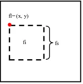
In Fig. 1, there are seven kinds of basic Haar feature types, each of them indicate their corresponding filtering box. The black heig_X. These basic features can be translated to position fl and scaled by factor fs within a patch as shown in Fig. 2. The solid outline represents the patch border, and the inside dashed rectangle represents the feature computation extent. This dashed rectangle can be translated, scaled within the patch and varied for the basic type of Haar features. Then fl can take any values so that the dashed line in Fig. 2 fits inside the patch for a given Haar feature type and fs is any natural number which is not larger than the min(FLOOR(wid_X/wid), F LOOR (heig_X/heig)). Within the patch X, each Haar feature f(X, fi, fs, fl) can be calculated very efficiently (Viola, Jones, 2004) using the integral image concept for patch X.
Fig. 2. The location fl, scale fs and feature type index fi of a Haar feature within a patch
The number of possible features K is the number of all possible combination of fl and fs for every fi. Note that different fi may have different fl and fs due to the varying basic size. We set wid_X = heig_X = 32, and take the first basic weak feature (fi= 1) as an example, the basic size is wid = heig = 2, and the largest scale is 16 (=min( FLOOR(32/2), FLOOR (32/2)). For each scale, the position fl has a different value range, the larger fs, the narrower is the value range of fl. For instance, if fs = 3, the value range of fl is {(x, y)| 1≤x≤27, 1≤y≤27}, which
ensures that the box lies completely inside the patch. Calculated in this manner, the whole number of combination over fi, fs, fl the number of weak classifiers is 124.2 million.
3.3 AdaBoost training
AdaBoost (Freund and Schapire, 1995) is used to train the response functions h. The learning algorithm works as follows:
Algorithm.1. AdaBoost training descriptors algorithm Input: M training patch pairs (Pi, li) containing both similar
and dissimilar patch pairs, where i∈{1,2...,M}. Dimensions of
descriptor D.
1) Initialize weights w1,i= 1 / M
2) for d=1:D
- Normalize weights so that the sum of weights is 1 - Select the best weak classifier that minimizes the
weighted matching error.
ei= 0 if sample i is classified correctly, ei= 1 otherwise. end
Output: Parameters: fd, θd, d, αd
The predicted label of matching is calculated as h(X1,i, f, θ)*
h(X2,i, f, θ), which is the product of two weak response values
on the same patch pairs. The initial weighting of different samples are the same, in each iteration we choose the best weak classifier that minimizes weighted matching error and update error. The weight updating decreases the weights of correctly classified samples and keeps the weights of incorrectly classified samples in the current iteration, so after weighting normalization in the next iteration, the weight of incorrect classification samples is higher. As a consequence, the next iteration of learning will focus on "difficult" samples.
The descriptor for patch X is C(X)= [h1(X) h2(X)... hD(X)] , where
Let (4) have a more general form
( , ) 1 classified as matching pairs, this improves the true positive rate but also leads to more non-matching patch pairs classified as matching pairs, which results in a higher false positive rate. Varying the threshold T means finding a trade-off between true positive rate and false positive rate.
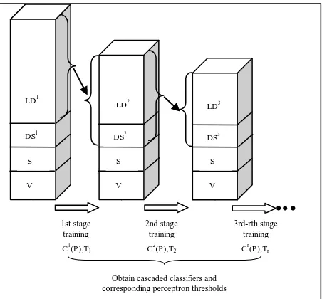
3.4 Cascade Classifier learning
Inspired by the work of (Viola, Jones, 2004), we propose a cascaded training and classification strategy for image matching. The training includes multiple training stages; each stage is trained by AdaBoost. The false positive samples from a large set of dissimilar patch pairs in the current stage are used to define
fs fl= (x, y)
fi
the negative training samples in the next stage. On the other hand, similar patches in training are fixed across all stages. This means that the training can see a huge number of negative examples which considers the fact that dissimilar patch pairs appear much more than similar patch pairs in a real matching scenario. The cascaded training algorithm is shown in algorithm 2, and a diagram of different sets changed in training is shown in Fig. 3. Here, the false positive rate (FPR) and the true positive rate (TPR) are defined towards the matching pairs. If a patch pair with the true label of similar is classified as similar, namely a matching pair, then it is predicted as a true positive result in our definition.
Algorithm 2. Cascaded classifier learning algorithm.
The final cascaded classifier works in the form of a decision list. Suppose the final learned classifier include S stages, to classify a patch pair, it will be classified as similar (matched) only if all AdaBoost classifiers in this decision list classify it as similar. A hidden benefit of this cascaded classification, as mentioned in (Viola, Jones, 2004), is that the number of negative training samples that the final algorithm sees can be very large. In later stages, the algorithm tends to concentrate on more difficult
Fig. 3. Multi-stage cascaded training from large dissimilar, similar, initial dissimilar and validation sets.
4. EXPERIMENTS
This section describes our experiments and the performance evaluation of our descriptor. First, we introduce the training data generation, and then we give some experiments of specific parameters in the descriptor learning process.
4.1 Training data
We use the Brown datasets (Brown et al., 2011b) in our experiments. This dataset includes three separate datasets - Notre dame, Yosemite and Liberty. The patches are centred on real interest points from the difference of Gaussian or Harris detectors. We first reduce the patch size from the original 64 by 64 pixels to 32 by 32 pixels. In each dataset, there are at least two patches from two or more different images for one interest point; the number of patches corresponding to one interest point. Suppose a specific interest point corresponds to Num_Patch patches, we choose the first patch as one patch and any of the following other Num_Patch-1 patches as its corresponding patch to form similar patch pairs. To generate dissimilar patch pairs, we randomly selected different interest point index pairs and select the patches also randomly from the patches to each
experiment, 5000 similar patch pairs and 5000 dissimilar patch pairs are used to train a descriptor with the algorithm described in 3.3. Different dimensions of trained classifiers are used to test the performance. The result is shown in Fig. 4.
It can be seen from Fig. 4 that when the dimension D of the descriptor becomes higher, the matching performance is improved, but the improvement slows down for D>60. The
LD: large dissimilar patch pair sets FPRtarget : target overall false positive rate
t: the minimum acceptable TPR in every layer S : similar patch pair sets for training. Its size is nS. DS: initial dissimilar patch pair sets. Its size is nDS 1) i= 0.
See equation (4) for defination of these parameters.
While TPR < t * TPRi-1
vary perceptron threshold T in (5) for the current strong classifier and compute the corresponding TPR on V.
dissimilar patch pairs for training of next stage. end While (FPRi > FPRtarget)
3) Record the number of stages Num_S= i. Output: Cascaded classifier { Cj
(P) | 1≤j≤Num_S} and
corresponding perceptron thresholds { Tj | 1≤j≤Num_S}.
V
in our experiments, which is roughly equal to a random guess. This kind of weak classifier barely contributes to the performance.
Fig. 4. ROC for descriptor learned at different dimensionality using 5000 similar + 5000 dissimilar samples
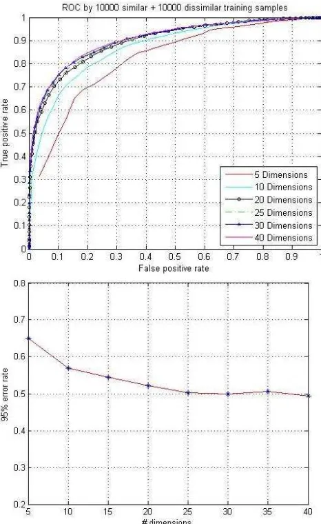
Fig. 5. ROC and 95% error rate for learned descriptor of different dimensionality using using 10000 similar + 10000
dissimilar samples
Another experiment for different dimensions and performance with 10000 similar and 10000 dissimilar patch pairs is given, achieving quite similar result. The result is shown in figure 5, which also presents the 95% error rate, which is the false positive rate when the true positive rate is 95%, for different dimensions D.
Fig. 5 also shows that the 95% error rate is relatively stable for D>25, and the ROC performance improves barely when using D>25. The descriptor resulting from using the first 25 dimensions can get very close in performance to the descriptor trained with the first 40 dimensions.
4.3 Cascaded AdaBoost descriptor learning
4.3.1 Cascaded Classifier Learning: To train the cascaded classifiers, we use 5000 positive and 5000 initial negative training samples, the large negative sets includes 700000 negative samples chosen from the Notre dame and Yosemite datasets. The validation set V includes 10000 positive and 10000 negative samples also chosen from the Notre dame and Yosemite datasets. Since the target true positive rate is 98% in every stage, the overall TPR goes down and it is impossible to get a 95% error rate. We use the accuracy as evaluation indicator. The trained cascaded classifier includes 12 stages. The change of TPR, FPR and accuracy on the validation set over different stages is listed in Fig. 6.
Fig. 6. TPR, FPR and Accuracy during training on validation set
From Fig. 6, we can see that the TPR decreases almost linearly, while the rate of descent for FPR is getting slower as the number of cascade stages increases. The whole accuracy reaches a steady level when using more than 8 stages.
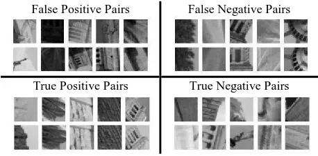
4.3.2 Performance Evaluation: To test the performance across datasets, we applied the trained cascaded classifier on test sets includes 5000 positive and 5000 negative samples which were randomly selected from the Liberty dataset. The confusion matrix is listed in table 1. As can been seen from the table, the recall for correct matches is 76.5%, while the overall accuracy is 86.0%.
Reference = + 1 Reference = -1 output = + 1 TP= 3827 FP= 224 output = -1 FN= 1173 TN= 4776
Table 1. Confusion matrix of cross dataset test for cascaded classification
Some of the randomly selected false positive, false negative, true positive and true negative patch pairs are shown in Fig. 7.
False Positive Pairs False Negative Pairs
True Positive Pairs True Negative Pairs
Fig. 7. Some cascaded classification result tested on Liberty set
5. CONCLUSION & FUTURE WORK
We have proposed a cascaded training and classification strategy for image matching. The feature pool is built on the threshold of response function for Haar features with different scales, and locations within the patch. The cascaded AdaBoost algorithm is used to train the classifier and descriptors at the individual shapes. In our cascaded learning framework, an order of 104 training samples is used in every stage, which leads to a classifier that is effective in 20 to 30 dimensions as shown in our experiment. Correspondingly, image matching is the process of going through a decision list. Only patch pairs reaching the final stage and classified as similar are accepted as successful matches in our algorithm. A potential drawback in our work is that the similarity measure used in this work lacks modelling the correlation between weak response functions.
In future research, we will compare the performance of our descriptor to classic descriptors. Additionally, we also intend to extend this descriptor learning directly on image intensity patches, instead of only on patches surrounding feature point, to make it more general.
ACKNOWLEDGEMENTS
The author Lin Chen would like to thank the China Scholarship Council (CSC), which supports his PhD study in Leibniz Universität Hannover, Germany. The authors would also like to thank Tobias Klinger, Ralph Schmidt and other colleagues for instructive discussions.
REFERENCES
Babenko, B., Dollár, P., and Belongie, S., 2007. Task specific local region matching. IEEE 11th International Conference on Computer Vision. 1-8.
Bay, H., Ess, A., Tuytelaars, T., et al., 2008. Speeded-up robust features (SURF). Computer Vision and Image Understanding, 110(3): 346-359.
Brown, M., Hua, G., Winder, S., 2011a. Discriminative learning of local image descriptors. IEEE Trans Pattern Anal Mach Intell, 33(1): 43-57.
Brown, M., Süstrunk, S., Fua, P., 2011b. Spatio-chromatic decorrelation by shift-invariant filtering. Proceeding IEEE Conf. Computer Vision and Pattern Recognition Workshops, 27-34.
Cai, H., Mikolajczyk, K., Matas, J., 2011, Learning linear discriminant projections for dimensionality reduction of image
descriptors. IEEE Trans Pattern Anal Mach Intell, 33(2): 338-352.
Calonder, M., Lepetit, V., Strecha, C., et al. 2010. Brief: Binary robust independent elementary features, European Conference on Computer Vision (ECCV) 2010, Springer Berlin Heidelberg, 778-792.
Freund, Y., Schapire, R. E., 1995. A desicion-theoretic generaliza- tion of on-line learning and an application to boosting. Computational learning theory. Springer Berlin Heidelberg, 23-37.
Ke, Y., Sukthankar, R., 2004. PCA-SIFT: A more distinctive representation for local image descriptors. Proceeding IEEE Conf. Computer Vision and Pattern Recognition, (2): II-506-II-513
Leutenegger, S., Chli, M., Siegwart, R. Y.. BRISK, 2011. Binary robust invariant scalable keypoints. IEEE 11th International Conference on Computer Vision: 2548-2555.
Lowe, D. G., 2004. Distinctive image features from scale-invariant keypoints. International Journal of Computer Vision, 60(2): 91-110.
Heikkilä, M., Matti, P., Cordelia, S., 2009. Description of interest regions with local binary patterns. Pattern Recognition, 42(3): 425-436.
Mikolajczyk, K., Cordelia, S., 2005. A performance evaluation of local descriptors. IEEE Trans Pattern Anal Mach Intell, 10(27): 1615-1630.
Rublee, E., Rabaud, V., Konolige, K., et al. 2011. ORB: an efficient alternative to SIFT or SURF. ICCV 2011, Proceeding IEEE Conf. International Conference on Computer Vision: 2564-2571.
Simonyan, K., Vedaldi, A., Zisserman, A., 2012. Descriptor learning using convex optimisation. European Conference on Computer Vision (ECCV) 2012. Springer Berlin Heidelberg, 243-256.
Strecha, C., Bronstein, A. M., Bronstein, M. M., Fua, P., 2012. LDAHash: Improved matching with smaller descriptors. IEEE Trans Pattern Anal Mach Intell, 34(1), 66-78.
Trzcinski, T., Christoudias, M., Lepetit, V., et al, 2012. Learning image descriptors with the boosting-trick. Advances in neural information processing systems:269-277.
Tola, E., Vincent, L., Fua, P., 2010. Daisy: An efficient dense descriptor applied to wide-baseline stereo. IEEE Trans Pattern Anal Mach Intell, 32(5): 815-830.
Viola, P., Jones, M. J., 2004. Robust real-time face detection. International Journal of Computer Vision, 57(2): 137-154. The International Archives of the Photogrammetry, Remote Sensing and Spatial Information Sciences, Volume XL-3, 2014