Impacts of stochastic models on real-time 3D UAV mapping
Muwaffaq Alqurashi a, *, Jinling Wang b
a
School of Civil and Environmental Engineering, UNSW Australia, Sydney 2052, Australia [email protected]
b
School of Civil and Environmental Engineering, UNSW Australia, Sydney 2052, Australia [email protected]
Commission VI, WG VI/4
KEY WORDS: 3D Mapping, Stochastic Model, Photogrammetry, Weight Matrix, Tie Point Measurements, Matching
ABSTRACT:
In UAV mapping using direct geo-referencing, the formation of stochastic model generally takes into the account the different types of measurements required to estimate the 3D coordinates of the feature points. Such measurements include image tie point coordinate measurements, camera position measurements and camera orientation measurements. In the commonly used stochastic model, it is commonly assumed that all tie point measurements have the same variance. In fact, these assumptions are not always realistic and thus, can lead to biased 3D feature coordinates. Tie point measurements for different image feature objects may not have the same accuracy due to the facts that the geometric distribution of features, particularly their feature matching conditions are different. More importantly, the accuracies of the geo-referencing measurements should also be considered into the mapping process. In this paper, impacts of typical stochastic models on the UAV mapping are investigated. It has been demonstrated that the quality of the geo-referencing measurements plays a critical role in real-time UAV mapping scenarios.
* Corresponding author. This is useful to know for communication with the appropriate person in cases with more than one author.
1. INTRODUCTION
Over the past decade, 3D mapping relying on the integration of Global Positioning System (GPS), Inertial Measurement Unit (IMU) and camera is commonly used. The integrated GPS/INS systems are used for direct geo-referencing purposes which allow the determination of the camera platform position and orientation with a high accuracy. The camera is utilised to provide the details of features for imaging. This basically reduces the need of ground control points (GCPs) by eliminating aerial-triangulation, except for mapping system calibrations (Grejner-Brzezinska and Toth, 2004). This in turn reduces the cost and the time for producing 3D digital maps. However, direct geo-referencing which obtains coordinates of ground objects directly using the known exterior orientation elements of photos is influenced by some error sources. These error sources such as interior and exterior orientation elements, errors of GPS, time synchronization and projection centre
deviation between GPS and vision sensors and errors of IMU degrade the accuracy and hence the efficiency of aerial photogrammetry (Zhang and Yuan, 2008).
Several studies have adopted a mathematical model which describes the relationship between measurements and unknown estimates (e.g., Wang et al, 2005) to eliminate the errors in aerial photogrammetry. On the other hand, stochastic model represents the statistical characteristics of the measurements. Such a stochastic model is mainly provided by the variance-covariance matrix for the measurements. If both models are defined correctly, optimal estimation can be achieved. The mathematical model has been addressed in different investigations in order to estimate the error sources in image
matching, POS (Position and Orientation System) or exterior orientation elements of images (e.g., Zhang and Yuan, 2008).
In 3D mapping using indirect geo-referencing, variance-covariance matrices are often constructed by the error propagation to present the precisions for the position and orientation of the camera, as well as the ground control points coordinates, which are treated error-free in the least-squares adjustments for the tie point coordinates (Marshall, 2012). In the adjustment, it is usually assumed that all tie point coordinates have the same precision. However, these assumptions are not always true due to different conditions such as their geometric distribution, and thus their feature matching environments. Therefore, it is necessary to construct a realistic stochastic model in order to achieve satisfactory geo-referencing and 3D mapping results. In this situation, different weights are assigned for each covariance matrix component which is basically preferred based on the standard deviation (Beinat and Crosilla, 2002). Thus, the covariance matrix is scaled by standard deviation factor (Goodall, 1991).
(2005) investigated the reliability in constrained Gauss-Markov model, which dealt with the measurements of the position and the orientation of the camera as uncorrelated measurements. In this study, it was also assumed that the horizontal positioning measurements of the camera have different precision from vertical positioning measurements. While more attention was more paid to investigating the precision of the exterior orientation elements of images, the precision of tie point measurements and the associated stochastic models have not been investigated in details yet.
In this paper, the precision of tie point measurements in stochastic model and its impact on 3D mapping will be addressed. In addition, the properties of the covariance matrix will be examined in order to provide a weight for tie points according to their geometric distribution. The rest of this paper is organised as follows. Section 2 deals with least squares in terms of functional and stochastic models for the UAV mapping, together with a new stochastic model for tie point coordinates. Section 3 presents and discusses numerical results, which will be followed with Section 4 for the concluding remarks.
2. LEAST SQUARES IN UAV MAPPING
2.1 Functional and stochastic models
The functional model, in general, describes the relation between the measured elements and the estimated elements. In photogrammetry, if the measured elements are image tie point coordinates with Cartesian coordinates, then the functional models could be (Cooper and Cross, 1988):
)
origin of the image coordinates and the true origin.f
= the focal lengthj
X
,Y
j,Z
j= object coordinates of pointj
c
X
,Y
c,Z
c= coordinates of projection centrem
= the elements of rotation matrixEquations 1 and 2 are known as collinearity equations which show the rigorous geometric relationships between the object coordinates, projection centre and image coordinates of the object. The functional model generally contains non-linear equations and the stochastic nature of the observations, which are considered as random variables, must be taken into account. The non-linear equations can be linearized by using Taylor relationships between ground and image coordinates of the object and the projection centre ;
x
= thet
1
vector of unknown parameters.The functional model can be an inaccurate description of the relationship between ground and image coordinates of the object due to gross (outlier), systematic (bias), and random errors. The gross errors can be a result of malfunction of instrument or an error in the software. These errors must be detected and removed before the estimation process. The second type of error is systematic errors. Camera lens distortions, light intensity, lack of orthogonality of the comparator axes, and atmospheric refraction are some physical effects that can cause the systematic errors (Cooper and Cross, 1988). The systematic errors cannot be removed, but there are two different ways to reduce their effects. Firstly, they can be considered in the functional model. For example, coordinates differences between the actual origin of the image coordinates and the true coordinates was dealt with as systematic errors and represented
in equations 1 and 2 as
x
o andy
o. Secondly, the biases areconsidered as stochastic effects which are accounted for by random parameters or by a priori correlation between the measurements. The third part of errors is the random errors which are usually unavoidable and bring small differences between the measurements and their expectations. Although they are uncertain, they follow statistical rules.
The stochastic model of least squares can be defined as:
1
= a priori variance factor being assigned as oneThe symbol P in equation (4) represents the weight matrix with n measurements.
where
2A= variance of tie point measurements2 measurements can be obtained as (Gruen, 1985):
Pl
which are the optimal estimates of the unknown parameters and the residuals, respectively, if the measurements are unbiased and the stochastic model is realistic.
The co-factor matrices for the estimated parameters and the residuals respectively, can be written as:
1
2.2 Factored stochastic model for tie point measurements
In the commonly used stochastic model, the variances of tie point observations 2
A
are assumed to be the same. However, this assumption is not always true due to different conditions such as geometric distribution of the features and their matching environments. Based on this fact, the tie point measurements should be given different weights. In this paper, the tie point measurements in x-axis are assigned different weight based on its distance from the x values of the camera position and the measurements in y-axis based on its distance from the y values of the camera position. This will reduce the effect of biases which have not been considered in the functional model. In addition, the proposed method of weighting of the tie point measurements is based on the assumption that the tie point measurements do not have any faulty measurements (outliers). The faulty measurements or mismatches are not discussed here and are treated in separate studies.
The investigation of the impact of the stochastic models on the accuracy of the object coordinates are carried with the commonly used model and the factored stochastic model as discussed below.
The equations used for determining the factor of tie point variance can be obtained as follows:
1
and
y
= the difference distance between object position and cameras positionX
andY
= the distance between the farthest object and the centreThus, the variances of each tie point can be computed as:
2 navigation and geo-referencing. The obtained images in digital form can provide the opportunity to process the data automatically. The GPS/INS systems can immediately deliver the geo-referencing information. The automatic process for obtaining geo-referencing information and for completing images matching gives the ability to generate 3D maps in real time to be used in military, scientific, and industrial applications. However, the quality of the real-time 3D mapping essentially relies on the accuracy of geo-referencing and matching results. So, the precision of the tie point, camera position and orientation measurements and their impacts on the 3D mapping will be analysed in the following sections.
3.1 Simulations
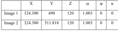
Two UAV images were simulated. They have longitudinal overlap and 15, 23, and 23 objects in the overlapped area.The first and the second simulations were completed with assuming all objects have the same height (zero) and the third simulation each object have different height but in the range between zero and 20 meters. Camera position in a local coordinate system and orientation are also identified Table 1. Tie point values are calculated and defined for each image. In the simulation, the focal length is assumed to be 24.47 (mm), sensor size (14.83 × 22.24), height flight 120 (meters), pixel size 6.44 μm, and the longitudinal overlap 70%.
X Y Z κ
Image 1 324.300 490 120 1.003 0 0
Image 2 324.300 511.818 120 1.003 0 0
3.2 The precision of tie point measurements and the standard deviations
Figure 1. Mapping Scenario 1: The horizontal positions of the tie-point objects
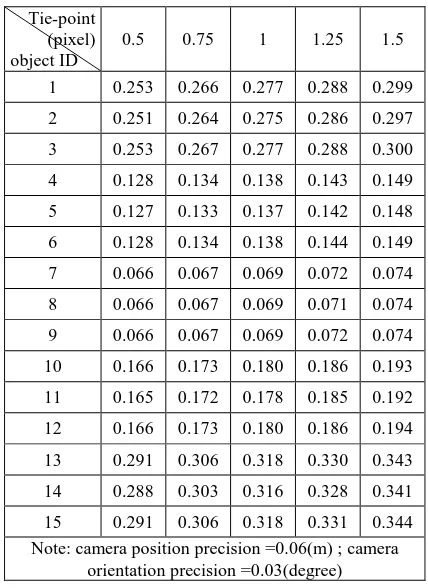
In this section, the impact of the precision of tie point measurements on the standard deviations of the estimated object coordinates has been investigated for Mapping Scenario 1 (Figure 1). The computation of the standard deviations for the object coordinates is completed with assuming that we have five levels of precision of the tie point measurements and the precision for the camera position and orientation pseudo-measurements are 6 cm and 0.03 degree respectively. It can be seen in Tables 2, 3, and 4 that the standard deviations in X, Y, and Z axes of the estimated parameters increase with the increase of the tie point precision vales from 0.5 to 0.75 pixels, from 0.75 to 1 pixel, from 1 to 1.25 pixels, and from 1.25 to 1.5 pixels.
From Table 2, it can be noted that the increase in the tie point precision values does not have the same impact on all objects. For example, the standard deviations in X-axis for objects 1, 2, and 3 increase more than 1 cm, whereas the increase for objects 7, 8, and 9 does not exceed 3 mm. Also, it can be seen that the standard deviations in X-axis of all objects in each level of the precision of tie point measurements are not the same. The standard deviations of objects 1, 2, and 3 can be categorised in one group in which the values of the standard deviations almost do not change (the maximum variation is 3 mm). The other objects can be in other groups as follows (4, 5, and 6), (7, 8, and 9), (10, 11, and 12), and finally (13, 14, and 15). From Figure 1, it can be noted that each group lie in the same position in X-axis.
Table 3 shows the standard deviations of the estimated parameters in Y-axis with different precisions of tie points. Similar to the standard deviation in X-axis, the standard deviations in Y-axis increase with the increase in the precision values and the magnitude of the increase depends also on object positions. It can also be noted that the values of the standard deviation for the objects (2, 5, 8, 11 and 14) lie on the centre differ significantly from the values of the other objects. This indicates the standard deviations values are not only affected by the precision of tie point measurements. The geometry also has an impact on the standard deviations.
Tie-point (pixel) object ID
0.5 0.75 1 1.25 1.5
1 0.253 0.266 0.277 0.288 0.299
2 0.251 0.264 0.275 0.286 0.297
3 0.253 0.267 0.277 0.288 0.300
4 0.128 0.134 0.138 0.143 0.149
5 0.127 0.133 0.137 0.142 0.148
6 0.128 0.134 0.138 0.144 0.149
7 0.066 0.067 0.069 0.072 0.074
8 0.066 0.067 0.069 0.071 0.074
9 0.066 0.067 0.069 0.072 0.074
10 0.166 0.173 0.180 0.186 0.193
11 0.165 0.172 0.178 0.185 0.192
12 0.166 0.173 0.180 0.186 0.194
13 0.291 0.306 0.318 0.330 0.343
14 0.288 0.303 0.316 0.328 0.341
15 0.291 0.306 0.318 0.331 0.344 Note: camera position precision =0.06(m) ; camera
orientation precision =0.03(degree)
Table 2. Impacts of tie point precision on the standard deviation in X-axis for Mapping Scenario 1
Tie-point (pixel) object ID
0.5 0.75 1 1.25 1.5
1 0.109 0.113 0.117 0.122 0.126
2 0.064 0.066 0.067 0.069 0.072
3 0.110 0.114 0.118 0.123 0.127
4 0.107 0.112 0.115 0.119 0.124
5 0.063 0.064 0.066 0.068 0.070
6 0.108 0.112 0.116 0.120 0.125
7 0.107 0.111 0.115 0.119 0.124
8 0.062 0.064 0.065 0.067 0.070
9 0.108 0.112 0.116 0.120 0.125
10 0.108 0.112 0.116 0.120 0.125
11 0.063 0.064 0.066 0.068 0.071
12 0.109 0.113 0.117 0.121 0.126
13 0.110 0.114 0.118 0.123 0.127
14 0.065 0.066 0.068 0.070 0.072
15 0.111 0.115 0.119 0.124 0.128 Note: camera position precision =0.06(m) ; camera
orientation precision =0.03(degree)
Table 3. Impacts of tie point precision on the standard deviation in Y-axis for Mapping Scenario 1
almost 3-3.5 cm. The geometry impact here is not clearly noted due to the fact that all objects in Mapping Scenario 1 have the same elevation. However, there are small differences because of the effect of the horizontal position. If we see the raise in the standard deviation of object 1 in the cases of 1.25 and 1.5 pixels, it is 3 cm. Similarly in object 8, the increase is 2.9 cm which does not differ significantly.
Tie-point (pixel) object ID
0.5 0.75 1 1.25 1.5
1 0.668 0.703 0.732 0.760 0.790
2 0.663 0.698 0.726 0.755 0.785
3 0.668 0.704 0.733 0.762 0.792
4 0.664 0.696 0.722 0.749 0.778
5 0.659 0.690 0.716 0.743 0.773
6 0.664 0.696 0.723 0.750 0.780
7 0.664 0.695 0.720 0.746 0.775
8 0.658 0.689 0.714 0.741 0.770
9 0.664 0.695 0.721 0.748 0.777
10 0.668 0.700 0.726 0.753 0.782
11 0.662 0.694 0.720 0.747 0.776
12 0.668 0.700 0.727 0.754 0.783
13 0.675 0.711 0.739 0.767 0.797
14 0.670 0.705 0.733 0.761 0.791
15 0.675 0.711 0.740 0.768 0.799 Note: camera position precision =0.06(m) ; camera
orientation precision =0.03(degree)
Table 4. Impacts of tie point precision on the standard deviation in Z-axis for Mapping Scenario 1
3.3 The precision of camera position pseudo-measurements and the standard deviations
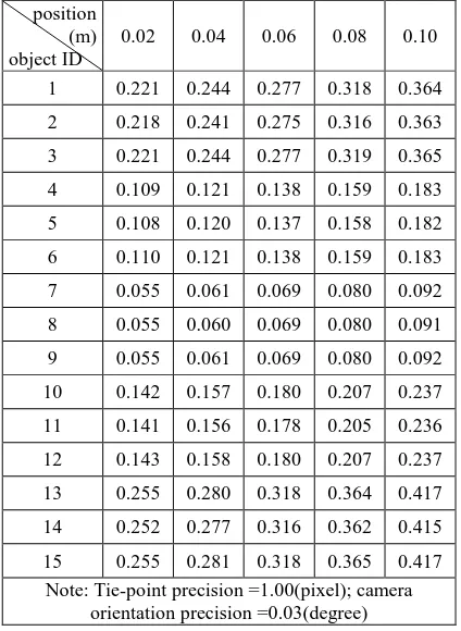
The impact of the precision of the camera position pseudo-measurements in Mapping Scenario 1 on the standard deviations is presented in Tables 5, 6, and 7. The assumed precision of the tie point is 1 pixel and the precision of the camera orientation is 0.03 degree. The precisions of the camera position are 2, 4, 6, 8, and 10 cm. Tables 5, 6, and 7 shows that the increase in camera position precision increases the standard deviation values in X, Y, and Z axes.
Table 5 illustrates the standard deviation values in X-axis under different cases of camera position precision. From Table 5, although the increase in the precision value in all cases is 2 cm, we can see that the increase in standard deviations is not the same. For example, the increase in the standard deviation of object 1 of the cases of 2 and 4 cm precision is 2.3 cm, whereas the increase of the cases of 8 and 10 cm is 4.6 cm. Similarly to what happened in the previous section, the geometry plays a role in the increase in the standard deviation values and in the standard deviation values themselves. For instance, the increase in the standard deviation of object 1 of the cases of 2 and 4 cm precision is 2.3 cm, while the increase in object 8 is 5 mm.
Table 6 shows the standard deviation values in Y-axis under different cases of camera position precision. It is clearly seen
that the increase in the precision value raises the standard deviation values. It can also be noted that the standard deviation values of the objects (2, 5, 8, 11, and 14) on the centre of Y-axis are about the half of the values for the other objects.
position (m) object ID
0.02 0.04 0.06 0.08 0.10
1 0.221 0.244 0.277 0.318 0.364
2 0.218 0.241 0.275 0.316 0.363
3 0.221 0.244 0.277 0.319 0.365
4 0.109 0.121 0.138 0.159 0.183
5 0.108 0.120 0.137 0.158 0.182
6 0.110 0.121 0.138 0.159 0.183
7 0.055 0.061 0.069 0.080 0.092
8 0.055 0.060 0.069 0.080 0.091
9 0.055 0.061 0.069 0.080 0.092
10 0.142 0.157 0.180 0.207 0.237
11 0.141 0.156 0.178 0.205 0.236
12 0.143 0.158 0.180 0.207 0.237
13 0.255 0.280 0.318 0.364 0.417
14 0.252 0.277 0.316 0.362 0.415
15 0.255 0.281 0.318 0.365 0.417 Note: Tie-point precision =1.00(pixel); camera
orientation precision =0.03(degree)
Table 5. Impacts of camera position precision on the standard deviation in X-axis for Mapping Scenario 1
position (m) object ID
0.02 0.04 0.06 0.08 0.10
1 0.093 0.103 0.117 0.135 0.154
2 0.054 0.059 0.067 0.077 0.088
3 0.094 0.104 0.118 0.136 0.155
4 0.091 0.101 0.115 0.133 0.153
5 0.052 0.058 0.066 0.076 0.087
6 0.092 0.102 0.116 0.134 0.154
7 0.090 0.100 0.115 0.133 0.152
8 0.051 0.057 0.065 0.075 0.086
9 0.091 0.101 0.116 0.134 0.154
10 0.092 0.101 0.116 0.134 0.153
11 0.052 0.058 0.066 0.076 0.087
12 0.092 0.102 0.117 0.135 0.154
13 0.095 0.104 0.118 0.136 0.155
14 0.055 0.060 0.068 0.078 0.088
15 0.095 0.105 0.119 0.137 0.156 Note: Tie-point precision =1.00(pixel); camera
orientation precision =0.03(degree)
Table 7 shows the standard deviations for Z coordinates with various precisions of the camera position. From Table 7, it can be seen that the vertical standard deviation of all objects does not considerably change, as they have the same elevation. In addition, we can see that with the precision of camera position of 8 cm, the standard deviation in object 1 is decreased by more than 12 cm compared to the case with 10 cm precision. This is not the same when the precision is changed from 4 to 2 cm. the decrease in the standard deviation in object 1 is only 6 cm. However, the impact of the increase in the precision value (2 cm) in the latter case which is 6 cm can be considered as big deviation that prevents from achieving more accurate results for real-time UAV 3D mapping.
position (m) object ID
0.02 0.04 0.06 0.08 0.10
1 0.583 0.643 0.732 0.841 0.963
2 0.576 0.637 0.726 0.835 0.958
3 0.584 0.644 0.733 0.841 0.963
4 0.571 0.632 0.722 0.832 0.955
5 0.564 0.625 0.716 0.827 0.950
6 0.572 0.633 0.723 0.833 0.956
7 0.568 0.630 0.720 0.830 0.953
8 0.561 0.623 0.714 0.825 0.949
9 0.569 0.631 0.721 0.831 0.954
10 0.576 0.636 0.726 0.835 0.958
11 0.569 0.630 0.720 0.830 0.953
12 0.577 0.637 0.727 0.836 0.959
13 0.592 0.651 0.739 0.847 0.968
14 0.585 0.645 0.733 0.842 0.963
15 0.593 0.652 0.740 0.847 0.968 Note: Tie-point precision =1.00(pixel); camera
orientation precision =0.03(degree)
Table 7. Impacts of camera position precision on the standard deviation in Z-axis for Mapping Scenario 1
3.4 The precision of camera orientation pseudo- measurements and the standard deviations
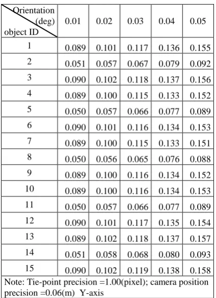
Tables 8, 9, and 10 illustrate the impact of the precision of the camera orientation pseudo-measurements on the standard deviations. The assumed precision of the tie point is 1 pixel and of the camera position is 6 cm. The standard deviations are computed under different scenarios of camera orientation precision (0.01, 0.02, 0.03, 0.04, and 0.05 degree). With the increase in the precision values, the standard deviation values increase.
Table 8 shows the standard deviations in X- axis for various cases of the precision of the camera orientation. It can be noted that the standard deviations in X-axis is affected by the increase in the precision values of the camera orientation and the distance from the centre of the X-axis. Furthermore, the objects on the same X-axis have almost the same standard deviation. The differences do not exceed few millimetres.
Orientation (deg) object ID
0.01 0.02 0.03 0.04 0.05
1 0.211 0.240 0.277 0.319 0.361
2 0.211 0.238 0.275 0.316 0.357
3 0.212 0.240 0.277 0.319 0.361
4 0.106 0.120 0.138 0.160 0.182
5 0.106 0.119 0.137 0.158 0.180
6 0.106 0.120 0.138 0.160 0.182
7 0.053 0.060 0.069 0.081 0.093
8 0.053 0.060 0.069 0.080 0.093
9 0.053 0.060 0.069 0.081 0.093
10 0.137 0.155 0.180 0.207 0.236
11 0.137 0.154 0.178 0.205 0.233
12 0.138 0.155 0.180 0.207 0.236
13 0.241 0.274 0.318 0.367 0.417
14 0.240 0.272 0.316 0.363 0.412
15 0.241 0.274 0.318 0.367 0.417 Note: Tie-point precision =1.00(pixel); camera position precision =0.06(m)
Table 8. Impacts of camera orientation precision on the standard deviation in X-axis for simulation 1
Orientation (deg) object ID
0.01 0.02 0.03 0.04 0.05
1 0.089 0.101 0.117 0.136 0.155
2 0.051 0.057 0.067 0.079 0.092
3 0.090 0.102 0.118 0.137 0.156
4 0.089 0.100 0.115 0.133 0.152
5 0.050 0.057 0.066 0.077 0.089
6 0.090 0.101 0.116 0.134 0.153
7 0.089 0.100 0.115 0.133 0.151
8 0.050 0.056 0.065 0.076 0.088
9 0.089 0.100 0.116 0.134 0.152
10 0.089 0.100 0.116 0.134 0.153
11 0.050 0.057 0.066 0.077 0.089
12 0.090 0.101 0.117 0.135 0.154
13 0.089 0.102 0.118 0.137 0.157
14 0.051 0.058 0.068 0.080 0.093
15 0.090 0.102 0.119 0.138 0.158 Note: Tie-point precision =1.00(pixel); camera position precision =0.06(m) Y-axis
Table 9. Impacts of camera orientation precision on the standard deviation in Y-axis for Mapping Scenario 1
standard deviation values. It can also be observed that the standard deviation values of the objects 2, 5, 8, 11, and 14 which are close to the centre of Y-axis are considerably smaller than the values for the other objects.
Table 10 shows the vertical standard deviations for five cases of the precision of the camera orientation. We can see that the standard deviation of all objects does not significantly vary, as their elevation is the same. In other words, the objects cannot be grouped as it can be done for the X-axis and Y-axis. The increase by 0.01 degree in the precision of the camera orientation can lead to an increase in standard deviation for some objects to more than 10 cm.
Orientation (deg) object ID
0.01 0.02 0.03 0.04 0.05
1 0.558 0.632 0.732 0.842 0.953
2 0.557 0.629 0.726 0.833 0.942
3 0.559 0.633 0.733 0.842 0.954
4 0.555 0.625 0.722 0.831 0.942
5 0.554 0.622 0.716 0.822 0.931
6 0.556 0.626 0.723 0.832 0.943
7 0.555 0.624 0.720 0.829 0.941
8 0.554 0.621 0.714 0.820 0.930
9 0.556 0.625 0.721 0.830 0.942
10 0.556 0.628 0.726 0.837 0.950
11 0.555 0.624 0.720 0.828 0.939
12 0.557 0.628 0.727 0.837 0.951
13 0.559 0.636 0.739 0.853 0.968
14 0.558 0.633 0.733 0.844 0.956
15 0.560 0.637 0.740 0.853 0.968 Note: Tie-point precision =1.00(pixel); camera position precision =0.06(m)
Table 10. Impacts of camera orientation precision on the standard deviation in Z-axis for Mapping Scenario 1
3.5 Horizontal positions of objects and the standard deviations for the tie point coordinates
Figure 2. Mapping Scenario 2: The horizontal positions of the tie-point objects
In Mapping Scenario 2 there were 23 tie point objects (Figure 2). These objects were utilised to generate tie point measurements. Knowing tie point measurements and camera parameters, 3D coordinates can be obtained through bundle block adjustment. The stochastic model was constructed with the assumptions that the tie point measurements assumed to have half pixel precision, camera positioning measurements have 5cm precision and camera orientation measurements are with 0.01 degree precision.
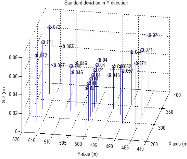
In addition to the 3D coordinates, the standard deviations of the object coordinates in 3D in the Mapping Scenario 2 were computed and presented in Figures (3, 4, and 5). In Figure (3) it can be seen that the standard deviation is the minimum in the centre of X-axis which is camera position in X-axis and increases with the distance from the centre. They are 0.04 m in the middle and increases in the left part to 0.06m then to 0.11 and finally to 0.16 m. On the right, they increase until they reach 0.17m. It is worth to mention that the objects No. (21, 22, and 23) are far from the centre about 45 m and the objects No. (1, 2, and 3) are 42 m. The standard deviations in Y-axis are minimum in the middle which is the average of camera positions in Y-axis when image 1 and image 2 captured. The values in the middle are 0.04 m and 0.071m in the farthest objects (Figure 4). It should be noted here that the distance between the farthest objects in Y-axis and the average positions of the camera is about 16 m. The standard deviations in Z-axis almost have the same values (Figure 5). This indicates that the variations in the standard deviations in Z-axis mainly depend on the vertical distance of the objects from the UAV height.
Figure 3. Standard deviations in X-axis for Mapping Scenario 2
Figure 5. Standard deviations in Z-axis for Mapping Scenario 2
3.6 Objects heights and standard deviations
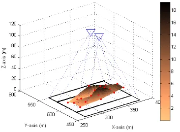
Mapping Scenario 3 was prepared with the same parameters in the Mapping Scenario 2 discussed above, but the only change was objects hieghts which were assigned randomly for the objects. It is important to remberer that the hights lay between 0 and 20 meters. This is because of the fact that the objects close to the boundaries of the images higher than 20 m may not be captured by the camera as shown in Figure 6.
Figure 6. The distributions of the tie point objects for Mapping Scenario 3
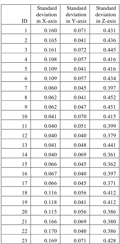
From Figures 7 and 8, it can be realised that the standard deviations in X-axis and Y-axis have the same situation obtained from the Mapping Scenario 2. However, the values are slightly affected by the hight variations of the objects. On the other hand, the standard deviations in Z-axis signicantly differ from the values in the Scenario 2 as shown in Figure 9.
Figure 7. Standard deviations in X-axis for Mapping Scenario 3
Figure 8. Standard deviations in Y-axis for Mapping Scenario 3
Figure 9. Standard deviations in Z-axis for Mapping Scenario 3
ID
Standard deviation in X-axis
Standard deviation in Y-axis
Standard deviation in Z-axis
1 0.160 0.071 0.431
2 0.165 0.041 0.436
3 0.161 0.072 0.445
4 0.108 0.057 0.416
5 0.109 0.041 0.416
6 0.109 0.057 0.434
7 0.060 0.045 0.397
8 0.062 0.041 0.452
9 0.062 0.047 0.451
10 0.041 0.070 0.415
11 0.040 0.051 0.399
12 0.040 0.040 0.379
13 0.041 0.048 0.441
14 0.040 0.069 0.361
15 0.066 0.045 0.362
16 0.067 0.040 0.397
17 0.066 0.045 0.371
18 0.116 0.056 0.412
19 0.118 0.041 0.412
20 0.115 0.056 0.386
21 0.166 0.069 0.380
22 0.170 0.040 0.386
23 0.169 0.071 0.428
Table 11. Standard deviations for Mapping Scenario 3 using the factored stochastic model
4. CONCLUSION
In a real-time 3D UAV mapping scenario, the standard deviation of the objects were computed using simulation data assuming different levels of precisions of tie point, camera position and orientation measurements. The standard deviations of the estimated parameters also were computed and investigated using commonly used and factored stochastic model.
This paper shows in details the impact of the precision of tie point, camera position and orientation measurements and the geometric distribution on 3D mapping results. It has been demonstrated that the tie-point objects which are closer to the centre between camera positions have smaller standard deviations than the objects that are farther. Also, this study has also presented the impact of commonly used and factored stochastic models on the standard deviation results. The initial results have shown that the factored stochastic model have a similar performance as the commonly used model, while the precisions of the geo-referencing measurements play a critical role in real-time 3D mapping scenarios.
In this paper the factored stochastic model for the tie point measurements was based on the horizontal positions of the objects. However, more complex stochastic models may be further investigated
ACKNOWLEDGEMENTS
REFERENCES
Beinat, A., and Crosilla, F., 2002. A generalized factored stochastic model for the optimal global registration of LIDAR range images. International Archives of Photogrammetry, Remote Sensing and Spatial Information Sciences, 34 (3B) (2002), pp. 36–39
Cooper, M., Cross, P. A., 1988. Statistical Concepts and Their Application in Photogrammetry and Surveying. Photogrammetric Record, 12(7 1): 637-663
Cothren, J., 2005. Reliability in Constrained Gauss-Markov Models: An Analytical and Differential Approach with Applications in Photogrammetry. Report 473, The Ohio State University, Columbus, Ohio
Goodall, C., 1991. Procrustes methods in the statistical analysis of shape. Journal Royal Statistical Society Series B-Methodological, 53(2), pp. 285-339.
Grafarend, E., Kleusberg, A., and Schaffrin, B. 1980. An introduction to the variance-covariance components estimation of Helmert type. Zeitschrift für Vermessungswesen, Konrad Wittwer GmbH, Stuttgart, Germany, 105(2), 129-137.
Grejner-Brzezinska, DA. and Toth, C. 2004. High accuracy direct aerial platform orientation with tightly coupled GPS/INS system. Report 147810, The Ohio State University,
Columbus, Ohio
Gruen, A. 1985. Adaptive Least Squares Correlation: A Powerful Image matching Techniques. Journal of Photogrammetry, Remote Sensing and Cartography 14 (3), 1985: 175-187
Marshall, J., 2012. Spatial Uncertainty in Line-Surface Intersections with Applications to Photogrammetry, ISPRS Annals of the Photogrammetry, Remote Sensing and Spatial Information Sciences, Volume I-2, 2012XXII ISPRS Congress, 25 August – 01 September 2012, Melbourne, Australia
Mohamed, A. H. and Schwarz, K. P. 1999. Adaptive Kalman Filtering for INS/GPS. Journal of Geodesy (1999) 73: 193-203
Quinchia, A. G., Falco, G., Falletti, E., Dovis, F., Ferrer, C., 2013. A Comparison between Different Error Modeling of MEMS Applied to GPS/INS Integrated Systems.Sensors. 13(8):9549-9588.
Rao, C. R., 1971. Estimation of variance and covariance components-MINQUE. Journal of Multivariate Analysis., 1, 257-275.
Wang, J., Stewart, M., and Tsakiri, M., 1998. Stochastic Modelling for Static GPS Baseline Data Processing, Journal of Surveying Engineering, 124, pp 171-181
Wang, J., Lee, H. K., Lee, Y., Musa, T and Rizos, C., 2005. Online Stochastic Modelling for Network-Based GPS Real-Time Kinematic Positioning, Journal of Global Positioning Systems Vol. 4, No. 1-2: 113-119
Wang, J., Wang. J., 2007. Adaptive tropospheric delay modelling in GPS/INS/Pseudolite integration for airborne surveying. The Journal of Global Positioning Systems, vol. 6, pp. 142 – 148