BLIND DECONVOLUTION ON UNDERWATER IMAGES FOR GAS BUBBLE
MEASUREMENT
C. Zelenka , R. Koch
Multimedia Information Processing, Dept. of Computer Science, Kiel University - (cze, rk)@informatik.uni-kiel.de
Commission V
KEY WORDS:Underwater, Image Processing, Measurement Techniques, Image Restoration, Blind Deconvolution
ABSTRACT:
Marine gas seeps, such as in the Panarea area near Sicily (McGinnis et al., 2011), emit large amounts of methane and carbon-dioxide, greenhouse gases. Better understanding their impact on the climate and the marine environment requires precise measurements of the gas flux. Camera based bubble measurement systems suffer from defocus blur caused by a combination of small depth of field, insufficient lighting and from motion blur due to rapid bubble movement. These adverse conditions are typical for open sea underwater bubble images. As a consequence so called ’bubble boxes’ have been built, which use elaborate setups, specialized cameras and high power illumination. A typical value of light power used is 1000W (Leifer et al., 2003).
In this paper we propose the compensation of defocus and motion blur in underwater images by using blind deconvolution techniques. The quality of the images can be greatly improved, which will relax requirements on bubble boxes, reduce their energy consumption and widen their usability.
1. INTRODUCTION
In areas like the Panarea area near Sicily (McGinnis et al., 2011) or the Tommelitten (Schneider von Deimling et al., 2011) in the North Sea, large amounts of carbon dioxide and methane are emitted from underwater gas seeps.
Because of the significance of underwater gas emissions on ma-rine life (Ishimatsu et al., 2004), (Dando and Hovland, 1992) and because of the impact on the climate, accurate measurements of the properties of the occurring gas bubbles are necessary, to be able to accurately estimate their impact (Liang et al., 2011). Dif-ferent ways to measure gas bubbles have been pursued in recent years. Most prevailing are acoustic (McGinnis et al., 2006) and optical measurement. We focus on camera based measurements, because they allow more accurate observations of gas bubbles. High quality images allow flow measurement with an error of less than 6 percent, as confirmed by practical tests (Zelenka, 2014).
Underwater imaging conditions are far from ideal for this kind of observations. They typically suffer from low light, due to power restrictions. The flamboyant bubbles can reach velocities of up to 25cm per second (Leifer et al., 2003). To prevent motion blur, high shutter speed and low integration times are necessary, which results in even less light on the image sensor (for detailed experi-ments see (Leifer et al., 2003)). Using a fast lens, which means a high aperture, is not a solution, because this lowers the depth of field and leads to potentially defocused images.
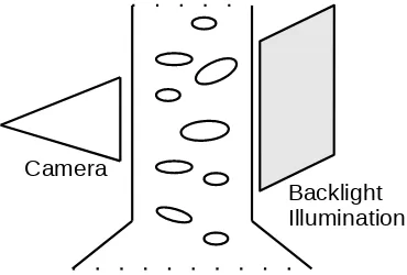
To overcome this problems, so called bubble boxes have been developed (Thomanek et al., 2010). A bubble box as shown in Figure 1 includes a camera, channeling elements to concentrate the bubbles in the cameras depth of focus, and a backlight illu-mination. Although front side illumination is known (Zielinski et al., 2010), for quantitative bubble measurement backlight illumi-nation is prevalent due to higher light efficiency and bubble rim visibility.
This does not solve the problem entirely, as strong lighting is still an issue, as the 1000 Watt illuminations in (Wang and Dong,
Camera
Backlight
Illumination
Figure 1: Drawing of a typical bubblebox
2009) and (Leifer et al., 2003) demonstrate. Because of the imag-ing conditions (see above), the bubble box also requires a high speed camera, such as in (Cheng and Burkhardt, 2006) (Leifer et al., 2003). Both requirements are costly and unwieldy in expedi-tion use.
Another factor often neglected in the literature is the presence of light scattering in the underwater ocean settings, caused by impu-rities in the water. This effect disturbs the light propagation and leads to blurry imaging and lowered accuracy, similar to defocus blur.
In this paper a different approach is developed, which is the ap-plication of suitable blind deconvolution techniques. The goal is not to avoid any blur or defocus, e.g. using high speed cameras and high power illuminations, but to compensate for these ef-fects. This allows a simplified buildup of a bubble box or images of higher quality in existing builds, while allowing more flexible experiments.
In this paper we focus on two different algorithms, the Richardson-Lucy standard algorithm and a more recent technique.
The Richardson-Lucy Algorithm by (Richardson, 1972) and (Lucy, 1974) with adaption to blind deconvolution by (Fish et al., 1995) is a fast standard deconvolution algorithm with a matlab imple-mentation (TheMathworks, 2015), which includes additional damp-ening. In recent years significant progress in the field of blind deconvolution has been made (Levin et al., 2011). Of particular interest are the gradient sparsity methods, because the gradient sparsity prior, which was originally established for natural im-ages, also applies very well on underwater gas bubble images. Which ideally consist of a uniform background with sparsely dis-tributed bubbles with high gradient rims.
We compare the heavy-tailed gradient sparsity MAP(Maximum a posteriori) blind deconvolution method by (Kotera et al., 2013) with the preceding standard technique and test whether they are suitable and applicable to underwater gas bubble images.
2. BLIND DECONVOLUTION TECHNIQUES
We model the observed imageOwith:
O=S∗B+n, (1)
whereSis the undisturbed signal disturbed byB, the blur kernel or point spread function (PSF) andnmodels added noise during the image formation. The aim of deconvolution algorithms is the reconstruction of the undisturbed signalSfrom the observation
O. If the PSF is unknown, a blind deconvolution algorithm with the added difficulty of estimating an unknownBis necessary.
We use blind deconvolution techniques, because the exact blur model of an underwater image is often unknown. Moreover mo-tion blur is dependent on bubble speed, the very parameter to be measured. Note that this reconstruction problem of two un-knowns from a single observation is inherently ill posed. A more in depth analysis of this problem can be found in (Levin et al., 2011) and (Perrone and Favaro, 2014).
The Richardson-Lucy deconvolution algorithm views this image formation model from a Bayesian perspective. For discrete event
A,Bwith an indexkandjthe Bayes theorem states:
P(A|B) = PP(B|A)·P(A)
An iterative algorithm with iteration indexiis defined by:
P(A)i+1=P(A)i
Applied to the deconvolution problem of Equation 1, this means associating the observed image OwithP(B), the undisturbed signalSwithP(A)and the blur kernelBwithP(B|A), similar to (Fish et al., 1995). In convolution notation this can be written as:
Si+1(x) =Si(x)
O(x)
Si(x)⊗B(x)
⊗B(−x). (5)
If the blur kernel is to be estimated, the analog update formula is:
Bi+1(x) =Bi(x) O
(x)
Bi(x)⊗S(x)
⊗S(−x). (6)
The Richardson-Lucy blind deconvolution algorithm (Fish et al., 1995) approaches the reconstruction problem of imageSand PSF
Bby alternating iterations in which the image and the PSF are re-fined. In this paper we use the standard matlab inplementation, which includes an additional dampening, to decrease noise prop-agation in the course of the iterations (TheMathworks, 2015).
In the following the blind deconvolution algorithm by (Kotera et al., 2013) is presented. It relies on a gradient sparsity prior that is maximized in the MAP(Maximum a posteriori)-estimation framework.
Given the Bayesian theorem and the image model Equation 1, neglecting noise, the goal is finding the MAP(Maximum A Pos-teriori) of
, whereP(S), etc. denote the probabilities and conditional prob-abilities ofO,S, andB, while assuming a Gaussian distribution with parameterµof
P(O|(S, B)) =∝e−µ2kS⊗B−Ok2. (8)
Q(S) and R(B) are regularizers of S and B respectively, to guide the optimization towards likely solutions. For the image
S the regularizerQregards the spatial gradientsDx andDyof
S:
withp∈(0,1)and indexiover the entirety of the partial deriva-tivesDxandDy. The variablepdefines the norm enforced on the gradients.
The blur kernelBis regularized with
R(B) =X
with the running indexiover allBiinBto enforce sparsity and non-negativity.
Instead of solving the MAP-problem directly, the negative loga-rithm of the target function is minimized, a common technique for MAP-estimation (Meintrup and Schaeffler, 2005). Constants are disregarded, because they do not influence the minimum:
In (Kotera et al., 2013) this optimization problem is solved using an augmented Lagrangian method in a multi-scale approach by alternatingly optimizing image and blur kernel.
3. APPLICATION AND RESULTS
In a laboratory setting a Point Grey Grasshopper 2 camera , back-light illumination and an air seep in a water tank are used in a similar build as shown in Figure 1 to obtain images of bubbles with varying acquisition parameters. The light power and camera setting such as focus, aperture and shutter speed are adjustable and provide a good foundation for experimentation with different kinds and strengths of blur. Images acquired with this system are used in the following.
3.1 Defocus blur
The two main sources of blur identified in a bubble box are defo-cus blur and motion blur.
First we will concentrate on defocus blur, which occurs if the bubbles are outside of the depth of field, centered at the focal plane. The depth of field determines the utility of the bubble me-ter, because it limits the distance range in which bubbles can be measured. A large depth of field requires a lens with a small aper-ture. However due to the difficult lighting conditions in underwa-ter settings discussed in the introduction, the aperture should be as large as reasonably possible. Solving this conflict by selecting an appropriate lens is a design decision requiring a compromise. In the following paragraph we show how the blind deconvolution techniques presented in the previous section apply to this setting and how they mitigate blur.
(a) Blurred original (b) Richardson-Lucy blind deconvolution result
(c) Gradient sparcity MAP Deconvolution result
Figure 2: Deconvolution of defocus blur. Both Richardson-Lucy and gradient sparsity MAP blind deconvolution achieve usable result, however the Richardson-Lucy method requires a good ini-tialization and shows inferior bubble edge sharpness.
A comparison of the results from Richardson-Lucy and gradient sparsity MAP-estimation (Kotera et al., 2013) on an image with mild defocus blur is shown in Figure 2 shows sharper edges and good deblurring. While the Richardson-Lucy algorithm is much faster, it suffers from strong ringing artifacts and increased noise. The restoration using MAP-estimation leads to much better re-sults, which less artifacts, less increase in noise and sharper bub-ble rims. Therefore it is our method of choice for the following experiments.
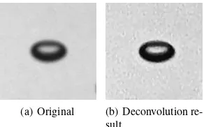
Using deconvolution on a noisy image as in Figure 3(a) reveals a negative property of the deconvolution. It increases the already present noise as shown in Figure 3(b).
(a) Original (b) Deconvolution re-sult
Figure 3: Noisy blurred image and its gradient sparsity deconvo-lution result.
3.2 Motion blur
Motion blur occurs if due to a combination of bubble motion and shutter speed, the light from a bubble is spread over several pixel. Choosing a very higher shutter speed, with a very short integra-tion time can solve this problem, but the light intensity avail-able for the image sensor is also determined by the integration time. Therefore this leads to dark and noisy images, unless a high power illumination is chosen.
In Figure 4 a series of images acquired with different shutter speeds is shown. In this image series automatic gain control to-gether with strong illumination and a large aperture lens were used to allow capturing images with constant brightness, even though the integration time differs significantly. Note that such a large aperture lens also negatively influences the depth of field. The left image was acquired with a very short integration time of only0.0004s, set by the camera control software, shows no mo-tion blur, while the image in the middle shows some momo-tion blur with an estimated blur radius of approx. 10pixel and the image on the right shows very strong motion blur with a blur radius of approx.15pixel.
(a) 0.0004s (b) 0.0020s (c) 0.0032s
Figure 4: Bubble images acquired with different integration times with automatic gain control.
While applying the deconvolution algorithm on images with dif-ferent intensities of motion blur, it becomes clear that there are limits to how strong the blur can be for the deconvolution to achieve a full compensation of the blur effects. We define a de-convolution successful only if the result is visually plausible and the blurred edges are fully restored without introducing artifacts, that may hinder an evaluation of the images.
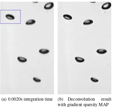
Figure 5 shows the deconvolution of image with medium motion blur, the same image as in Figure 4(b). The rim of the deconvolu-tion result is sharp, and resembles the low integradeconvolu-tion time image in Figure 4(a).
(a) 0.0020s integration time (b) Deconvolution result with gradient sparsity MAP
Figure 5: Medium motion blur image and gradient sparsity de-convolution. The dotted blue rectangle shows the cropped seg-ment of Figure 6.
(a) Original (b) Deconvolution result
(c) Snake segmentation on original image.
(d) Snake segmentation on deconvolution image
Figure 6: Measuring the bubble size with the snake algorithm. The initialization is shown in green, the snake is shown in red, while the fitted ellipse in blue.
deconvolution from 42 pixel to 37 pixel. This change is expected as blur around the rim of the bubble is removed, although the result is not as good as in artificial images (see Figure 9) and the restored contour could be even smaller.
Furthermore we measure the bubble size with automated algo-rithms (Zelenka, 2014). The different steps of the bubble segmen-tation are shown in Figures 6(c,d). A snake, an active contour, is initialized with the green bounding rectangle and iteratively contracts towards higher image gradients under smoothness con-straints. The final state of the snake is shown in red. To accurately measure the size the blue ellipse is fitted into the snake. The auto-matically measured bubble size remains constant with approx. 38 pixel height, which is confirmed by the segmentations in Figure 6. The weak blur on the outer rim of the bubble is disregarded and does not disturb the image gradient based algorithm, which is robust enough to cope with this blur.
For stronger motion blur shown in Figure 7 and Figure 8 the mo-tion blur is too strong to be removed with a same parameters used in Figure 5. On the original image, the snake method fails to ini-tialize and attempts to use multiple snakes for a single bubble (see Figure 8) and due to the blur even a manual size measurement is
hard. The deconvolution with standard parameters does not fully restore the original edges but creates new edges further around the bubble.
Changing the deconvolution parameters, allowing a larger PSF and weighting the blur kernel regularization in the blur kernel estimation the 2.5 times more than the data term, compensates the stronger blur (see Figure 7). It restores the sharp rim of the bubbles, similar in sharpness to non-blur image in Figure 4(a) and allows an accurate automatic measurement as in Figure 8. Because of this advantage, we think that the strong deconvolution artifacts, apparent by the white halo around the bubbles, can be tolerated.
(a) 0.0032s integration time (b) Deconvolution result with gradient sparsity MAP
Figure 7: Strong motion blur image and gradient sparsity decon-volution with changed weighting on the regularization allowing a more flexible blur kernel. The dotted blue rectangle shows the cropped segment of Figure 8.
(a) Original (b) Deconvolution result
(c) Failed segmentation of the original image
(d) Segmentation of the de-convolution image
Figure 8: Snake based measurement of a bubble from Figure 7, colors as in Figure 6.
(a) Original image (b) Artificial motion blurred image
(c) Deconvolution result of image (b)
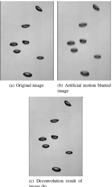
Figure 9: Comparison between original, blurred image and gradi-ent sparsity MAP deconvolution result for gas bubbles with 6mm diameter in a bubble box with back illumination. This demon-strates the accuracy of the deconvolution.
demonstrates that a successful deconvolution with gradient spar-sity MAP can provide an accurate restoration of the non-blurred image and can therefore be used for further evaluation.
4. CONCLUSIONS
In our experiments we have observed, how motion and defocus blur can influence the image and how deconvolution can restore them. Blur can lead to an overestimation of the bubble size or prevent automatic bubble measurements.A high measurement ac-curacy is necessary, because the bubble radius influences the vol-ume with the third power and bubble shape parameters like ellip-ticity are important to gas dissolution models like (McGinnis et al., 2006) and (Liang et al., 2011).
The two different algorithms showed a strong difference in per-formance. The standard blind Richardson-Lucy deconvolution, provided a good initialization, shows acceptable results for small defocus blur, even though ringing artifacts occur. The gradient sparsity MAP deconvolution can compensate much stronger blur and even some motion blur without artifacts. For strong motion blur, strong restoration artifacts have to be accepted.
Nevertheless with deconvolution, on images which could not be evaluated beforehand, the blur is removed, sharp contours are re-stored and the automatic evaluation is enabled. This allows clear measurements and lowered overestimation, which are strong ad-vantages. The complete potential of applying blind deconvolu-tion on bubble images is shown in the results seen in the compen-sation of artificial motion blur.
In case of non-changing conditions, such as bubble speed and wa-ter paramewa-ters, the restored blur kernel varies little. If the imag-ing conditions allow it, we propose usimag-ing the blind-deconvolution every few images to reconstruct the blur kernel from an initial image and reuse it for in the following images. This means for the consecutive images only non-blind deconvolution is required and the computational costs can be significantly reduced. The gradient sparsity MAP deconvolution takes9son the image in Figure 2, while the non-blind deconvolution Richardson-Lucy al-gorithm with the blur kernel set by the blind deconvolution is much faster with1s.
Currently only spatially invariant blur is considered. For future work, a spatially variant blur kernel estimation could be benefi-cial, because although the motion blur of the bubble in an image is similar in direction and magnitude, due to the variations in bub-ble motion it is not identical. Furthermore, with a small depth of field not all bubbles are in focus and a bubble may even change between focus and defocus over time. As future work, this means that the blur model could be estimated for every bubble individu-ally and incorporated or partiindividu-ally derived from the measured bub-ble motion.
In summary, we show in this paper, that blind deconvolution gives significant improvements in image quality and extends the usable depth of field in an underwater environment. We see that a certain amount of motion and defocus blur can be permitted with decon-volution, while maintaining high measurement accuracy . The compensation of image blur caused by defocus and motion per-mits more accurate flow measurements and relaxed requirements on underwater observatory equipment. This allows the design of a bubble box with higher measurement accuracy in a simplified setup, larger effective depth of field, and due to a higher tolerance to motion blur, less powerful illumination and camera.
REFERENCES
Cheng, D.-c. and Burkhardt, H., 2006. Template-based bub-ble identification and tracking in image sequences. International Journal of Thermal Sciences 45(3), pp. 321–330.
Dando, P. and Hovland, M., 1992. Environmental effects of sub-marine seeping natural gas. Continental Shelf Research 12(10), pp. 1197–1207.
Fan, F., Yang, K., Fu, B., Xia, M. and Zhang, W., 2010a. Appli-cation of blind deconvolution approach with image quality met-ric in underwater image restoration. In: image analysis and sig-nal processing (IASP), 2010 internatiosig-nal conference on, IEEE, pp. 236–239.
Fan, F., Yang, K., Xia, M., Li, W., Fu, B. and Zhang, W., 2010b. Comparative study on several blind deconvolution algorithms ap-plied to underwater image restoration. Optical review 17(3), pp. 123–129.
Fish, D. A., Brinicombe, A. M., Pike, E. R. and Walker, J. G., 1995. Blind deconvolution by means of the RichardsonLucy al-gorithm. Journal of the Optical Society of America A 12(1), pp. 58.
Ishimatsu, A., Kikkawa, T., Hayashi, M., Lee, K.-S. and Kita, J., 2004. Effects of CO2 on marine fish: larvae and adults. Journal of oceanography 60(4), pp. 731–741.
Leifer, I., de Leeuw, G. and Cohen, L. H., 2003. Optical Mea-surement of Bubbles: System Design and Application. J. Atmos. Oceanic Technol. 20(9), pp. 1317–1332.
Levin, A., Weiss, Y., Durand, F. and Freeman, W. T., 2011. Un-derstanding Blind Deconvolution Algorithms. IEEE Transactions on Pattern Analysis and Machine Intelligence 33(12), pp. 2354– 2367.
Liang, J.-H., McWilliams, J. C., Sullivan, P. P. and Baschek, B., 2011. Modeling bubbles and dissolved gases in the ocean. Journal of Geophysical Research 116(C3), pp. C03015.
Lucy, L. B., 1974. An iterative technique for the rectification of observed distributions. The Astronomical Journal 79, pp. 745.
McGinnis, D. F., Beaubien, S. E., Bigalke, N., Bryant, L., Celussi, M., Comici, C., De Vittor, C., Feldens, P., Giani, M., Karuza, A. and Schneider von Deimling, J., 2011. The Panarea natural CO2 seeps : Fate and impact of the leaking gas (PaCO2). Eurofleet’s Cruise Report U10, GEOMAR Helmholtz Centre for Ocean Research, Kiel.
McGinnis, D. F., Greinert, J., Artemov, Y., Beaubien, S. E. and West, A., 2006. Fate of rising methane bubbles in stratified wa-ters: How much methane reaches the atmosphere? Journal of Geophysical Research 111(C9), pp. C09007.
Meintrup, D. and Schaeffler, S., 2005. Stochastik. Springer, Berlin, Heidelberg.
Perrone, D. and Favaro, P., 2014. Total Variation Blind Decon-volution: The Devil Is in the Details. In: Computer Vision and Pattern Recognition (CVPR), 2014 IEEE Conference on, IEEE, pp. 2909–2916.
Richardson, W. H., 1972. Bayesian-Based Iterative Method of Image Restoration. Journal of the Optical Society of America 62(1), pp. 55.
Schneider von Deimling, J., Rehder, G., Greinert, J., McGinnnis, D., Boetius, A. and Linke, P., 2011. Quantification of seep-related methane gas emissions at Tommeliten, North Sea. Continental Shelf Research 31(7-8), pp. 867–878.
TheMathworks, 2015. Matlab documentation on blind deconvo-lution: www.mathworks.com/help/images/deblurring-with-the-blind-deconvolution-algorithm.html (9. Mar. 2015).
Thomanek, K., Zielinski, O., Sahling, H. and Bohrmann, G., 2010. Automated gas bubble imaging at sea floor a new method of in situ gas flux quantification. Ocean Sci. 6(2), pp. 549–562.
Wang, H. Y. and Dong, F., 2009. A method for bubble volume calculating in vertical two-phase flow. J. Phys.: Conf. Ser. 147(1), pp. 012018.
Wu, J.-L., Chang, C.-F. and Chen, C.-S., 2013. An Adaptive Richardson-Lucy Algorithm for Single Image Deblurring Using Local Extrema Filtering. Journal of Applied Science and Engi-neering 16(3), pp. 269–276.
Zelenka, C., 2014. Gas Bubble Shape Measurement and Analy-sis. In: Pattern Recognition, Lecture Notes in Computer Science, Springer International Publishing, pp. 743–749.