CALIBRATION AND ACCURACY ANALYSIS OF A FOCUSED PLENOPTIC CAMERA
N. Zellera, c,∗, F. Quintb, U. Stillac
aInstitute of Applied Research (IAF), Karlsruhe University of Applied Sciences, 76133 Karlsruhe, Germany - [email protected]
b
Faculty of Electrical Engineering and Information Technology, Karlsruhe University of Applied Sciences, 76133 Karlsruhe, Germany - [email protected]
c
Department of Photogrammetry and Remote Sensing, Technische Universitaet Muenchen, 80290 Munich, Germany - [email protected]
Commission III
KEY WORDS:Accuracy, calibration, depth map, imaging model, plenoptic camera, Raytrix, virtual depth
ABSTRACT:
In this article we introduce new methods for the calibration of depth images from focused plenoptic cameras and validate the results. We start with a brief description of the concept of a focused plenoptic camera and how from the recorded raw image a depth map can be estimated. For this camera, an analytical expression of the depth accuracy is derived for the first time. In the main part of the paper, methods to calibrate a focused plenoptic camera are developed and evaluated. The optical imaging process is calibrated by using a method which is already known from the calibration of traditional cameras. For the calibration of the depth map two new model based methods, which make use of the projection concept of the camera are developed. These new methods are compared to a common curve fitting approach, which is based on Taylor-series-approximation. Both model based methods show significant advantages compared to the curve fitting method. They need less reference points for calibration than the curve fitting method and moreover, supply a function which is valid in excess of the range of calibration. In addition the depth map accuracy of the plenoptic camera was experimentally investigated for different focal lengths of the main lens and is compared to the analytical evaluation.
1. INTRODUCTION
The concept of a plenoptic camera already has been developed more than hundred years ago (Ives, 1903, Lippmann, 1908). Nev-ertheless, only for the last few years the existing graphic pro-cessor units (GPUs) are capable to evaluate the recordings of a plenoptic camera with acceptable frame rates (≥30fps).
Today, there exist basically two concepts of a plenoptic camera which use a micro lens array (MLA) in front of the sensor. Those two concepts are the ”unfocused” plenoptic camera developed by Ng (Ng, 2006) and the focused plenoptic camera, which was de-scribed for the first time by Lunsdaine and Georgiev (Lunsdaine and Georgiev, 2008). The focused plenoptic camera can also be found as plenoptic camera 2.0 in the literature. One big advan-tage of it compared to the ”unfocused” plenoptic camera is the high resolution of the synthesized image. This is beneficial for estimating a depth map out of the recorded raw image (Perwass and Wietzke, 2012).
A camera system which is supposed to be use for a photogram-metric purpose has to be calibrated to transform the recorded im-ages to the metric object space. While in (Dansereau et al., 2013) the calibration of a Lytro camera (Ng, 2006) is described, (Jo-hannsen et al., 2013) presents the calibration of a Raytrix cam-era (Perwass and Wietzke, 2012) for object distances up to about
50cm. The methods presented here were also developed to cal-ibrate a Raytrix camera. Nevertheless, we are focused on de-veloping calibration method for farther object distances then the method described in (Johannsen et al., 2013).
This paper presents an analytical analysis of the depth accuracy which cannot be found in the literature until now. Afterwards, the developed calibration methods are presented. The presented
∗Corresponding author.
methods are separated into the calibration of the optical imag-ing process while disregardimag-ing the depth information and into the calibration of the depth map supplied by the camera. For the calibration of the depth map we present two newly developed ap-proaches and compare them to an already known method. All three methods are evaluated for different camera setups in a range of approx.0.7m to5m.
Different from (Johannsen et al., 2013) we did not investigate the distortion of the depth map by the main lens. However, for the focal lengths used in this article and for the large object distances we are operating with, the depth map distortion can be neglected compared to the stochastic noise of the depth information.
All experiments presented in this paper were performed using the camera Raytrix R5. In these experiments the impact of different focal lengths of the main lens on the depth information was an-alyzed and the different calibration methods were compared to each other.
This article is organized as follows. Section 2 presents the con-cept of a focused plenoptic camera. Here, we also derive the analytical expression for the accuracy of the depth map. In Sec-tion 3 the calibraSec-tion of the image projecSec-tion as well as the three depth calibration methods are presented. Section 4 presents ex-periments which were performed to evaluate the developed cali-bration methods and Section 5 shows the corresponding results.
2. CONCEPT OF THE CAMERA
fL fL
bL aL
main lens
Figure 1: Optical path of a thin lens
al., 1996) it is shown that in free space it is sufficient to define the light-field as a 4D function. Since the intensity along a ray does not change in free space, a ray can be defined by two position and two angle coordinates. From the recorded 4D light-field a depth map of the scene can be calculated or images focused on different object distances can be synthesized after recording.
Since this article describes the calibration of a Raytrix camera, only the concept for this camera is presented here. Neverthe-less, the existence of other concepts (Ng, 2006, Lunsdaine and Georgiev, 2008) has to be mentioned.
Figure 1 shows the projection of an object which is in the distance
aLin front of a thin lens to the focused image in a distancebL behind the lens. The relationship between the object distanceaL and the image distancebLis defined by the thin lens equation as given in eq. (1).
1 fL
= 1 aL
+ 1 bL
(1)
In eq. (1)fLis the focal length of the main lens.
The easiest way to understand the principle of a plenoptic camera is to look behind the main lens. Figure 2 shows the path of rays inside a Raytrix camera. There, the sensor is not arranged on the imaging plane, which is in the distancebLbehind the main lens, like it is for a traditional camera. In a Raytrix camera the sensor is placed closer thanbLto the main lens. Besides, in front of the sensor a MLA is assembled which focuses the virtual main lens image on the sensor. One distinct feature of Raytrix cameras is that they have MLAs which consist of micro lenses with three dif-ferent focal lengths. Each type of micro lenses focuses a difdif-ferent image distance on the sensor. Thus, the depth of field (DOF) of the synthesized image is increased by a factor of three.
The following Section 2.1 explains, how a depth map can be cal-culated based on the recorded raw image. For this description the MLA is assumed to be a pinhole grid which simplifies the path of rays. Nevertheless, within the DOF of the camera this assumption is valid. In this article the image synthesis will not be described. A detailed description can be found in (Perwass and Wietzke, 2012).
2.1 Calculating the depth map
As one can see from Figure 2, each of the three middle micro lenses projects the virtual main lens image, which would occur behind the sensor, on the sensor. Each micro image (image of a micro lens) which is formed on the sensor shows the virtual main lens image from a slightly different perspective. Based on the focused image of a point in two or more micro images the distance between the MLA and the virtual main lens imagebcan be calculated by triangulation (see Fig. 2 and 3).
Figure 3 shows how the distance between any virtual image point and the MLAbcan be calculated based on its projection in two
B bL0
b
fL
bL
D
D
D DL
main lens sensor
MLA
Figure 2: Optical path inside a Raytrix camera
px1
px2
d1
d2
d
B
b
sensor MLA
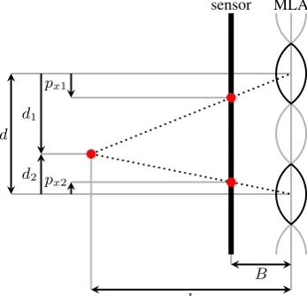
Figure 3: Principle of depth estimation in a Raytrix camera. The distancebbetween a virtual main lens image point and the MLA can be calculated based on its projection in two or more micro images.
micro images. In this figurepxi(fori∈ {1,2}) defines the dis-tance of the points in the micro images to the principal point of the respective micro image. Besides,di(fori∈ {1,2}) defines the distance of the respective principal point to the orthogonal projection of the virtual image point to the MLA. All distances
pxi, as well asdiare defined as signed values. Thus, distances with an upwards pointing arrow in Figure 3 are positive values and those with an downwards pointing arrow are negative val-ues. Triangles which have equal angles are similar and thus, the following relations hold:
pxi
B =
di
b −→ pxi=
di·B
b for i∈ {1,2} (2)
Besides, the base line distance between the two micro lenses can be calculated as given in eq. (3).
d=d2−d1 (3)
If we define the parallax of the virtual image pointpxas the dif-ference betweenpx2andpx1from eq. (2) and (3) the definition given in eq. (4) is received.
px=px2−px1 =
(d2−d1)·B
b =
d·B
b (4)
point and the MLAbcan be described as a function of the base line lengthd, the distance between MLA and sensorB, and the estimated parallaxpx, as given in eq. (5).
b=d·B px
(5)
A point occurs in more or less micro images depending on the distance of its virtual image to the MLA. Thus, dependent on this distance, the length of the base lined, which is used for triangu-lation, changes. If the triangulation would be performed by using two neighbored micro images, the based line would be equivalent to the micro lens aperture (d =D). Since in a Raytrix camera two neighbored micro lenses have different focal lengths, they never focus the same point on the sensor and thus, the baseline is always greater than the micro lens aperture (d > D).
The distanceBbetween sensor and MLA is not known exactly, thus, the depth map which is supplied by the plenoptic camera is the distancebdivided byB. This relative depth value is called virtual depth and is denoted byv. From eq. (5) the virtual depth
vas a function of the estimated parallax px and the base line distancedcan be derived, as given in eq. (6).
v= b
B =
d px
(6)
The virtual depth can only be calculated for a point which occurs focused in at least two micro images. Thus, caused by the hexa-gonal arrangement of the MLA with three different focal lengths, as it is in a Raytrix camera, a minimum measurable virtual depth ofvmin = 2results (Perwass and Wietzke, 2012). Since one point usually occurs focused in more than two micro images, its parallax can be estimated by using more than two images.
2.2 Depth accuracy
Based on the rules know from the theory of propagation of un-certainty one can see how an error of the estimated parallax will effect the depth accuracy. From the derivative ofvwith respect to the measured parallaxpxthe standard deviation of the virtual depthσvcan be approximated as given in eq. (7).
σv≈
From eq. (7) it is obtained that the accuracy of the virtual depth decays proportional tov2
. The base line distancedis a discon-tinuous function of the virtual depthv, because depending on the virtual depthvof a point the maximum base line length of micro lenses which see this point changes. This finally leads to a dis-continuous dependency of the depth accuracy as function of the object distanceaL. However, on average the base line distanced is proportional to the virtual depthv. So in total the accuracy of the virtual depth decays approximately proportional tov.
The relationship between the image distancebLand the virtual depthvis defined by the linear function given in eq. (8).
bL=b+bL0=v·B+bL0 (8)
HerebL0is the unknown but constant distance between main lens and MLA. Using the thin lens equation (1) one can finally express the object distanceaLas function of the virtual depthv. If the derivative ofaLwith respect tobLis calculated, the standard de-viation of the object distanceσaLcan be approximated as given
in eq. (9).
For object distances which are much higher than the focal length of the main lensfLthe approximation in eq. (9) can be further simplified as given in eq. (10). From eq. (10) one can see, that for a constant object distanceaLthe depth accuracy increases proportional tof2
L.
For a constant focal length of the main lens the depths accuracy decays proportional witha2
L. But, since large object distances are equivalent to a small virtual depth, the depth accuracy as a function of the object distanceaLis of better nature than given in eq. (10).
3. METHODS OF CALIBRATION
This section presents the developed methods to calibrate the fo-cused plenoptic camera. We divide the calibration into two sepa-rate parts. In the first part we calibsepa-rate the optical imaging process disregarding the estimated depth map. The second part addresses the calibration of the depth map.
3.1 Calibration of the optical imaging
For the calibration of optical imaging process the synthesized im-age is considered to result from a central projection, as it is also done for regular cameras. The intrinsic parameters of the pin-hole camera and the distortion parameters are estimated by the calibration method supplied by OpenCV. This method is mainly based on the approach described in (Zhang, 1999). Only the lens distortion model is the one described in (Brown, 1971).
This calibration method uses a number of object points on a plane which are recorded from many different perspectives. The pro-jection from an object point on the plane to the corresponding image point can be described by a planar homography as given in eq. (11). Here, the object point coordinates are denoted by
xW andyW whilezW = 0and the image point coordinates are
From the planar homography, which has to be estimated for each perspective, eight independent equations are received. From those eight equations six extrinsic parameters have to be calculated. Thus, from each perspective two equations are left to estimate the intrinsic parameters. Since OpenCV defines a pinhole camera model with four intrinsic parameters, the object points have to be recorded from at least two different perspectives. Those four in-trinsic parameters are the focal lengths of the pinhole camera in
After the determination of the intrinsic parameters, the distortion parameters can be estimated out of the difference between the projection of the object points on the image plane using the es-timated extrinsic and intrinsic parameters and the corresponding measured image points.
Based on the corrected image points, again the extrinsic and in-trinsic parameters are estimated. This procedure is repeated until consistency is reached.
3.2 Calibration of the depth map
Purpose of the depth map calibration is to define the relationship between the virtual depthvsupplied by the Raytrix camera and a metric dimensionowhich describes the distance to an object.
As described in Section 2 the relationship between the virtual depthvand the object distanceaLrelies on the thin lens equation, which is given in eq. (1). Nevertheless, a real lens usually can not be described properly by an ideal thin lens. Thus, for instance the position of the lens’ principal plane is not known exactly or the lens conforms to a thick lens with two principal planes.
From Figure 2 one can see, that the image distancebLis linearly dependent on the virtual depthv. This dependency is defined as given in eq. (12).
bL=v·B+bL0 (12)
Since the position of the main lens’ principal plane cannot be de-termined, the object distanceaLcannot be measured explicitly. Hence, the object distanceaLis defined as the sum of a measur-able distanceoand a constant but unknown offsetaL0as given in eq. (13).
aL=o+aL0 (13)
The definitions for the image distance bL and the object dis-tanceaL (eq. (12) and (13)) are inserted in the thin lens equa-tion (eq. (1)). After rearranging the thin lens equaequa-tion with the inserted terms, the measurable object distanceois described as a function of the virtual depthvas given in eq. (14).
o=
1 fL
− 1
v·B+bL0 −1
−aL0 (14)
This function depends on four unknown but constant parameters (fL,B,bL0, andaL0). The defined function between the virtual depthvand the measurable object distanceohas to be estimated. This estimation can be performed from a bunch of measured cal-ibration points for which the object distanceois known. In this paper we present two novel model based calibration methods. For comparison the function will also be approximated by a tradi-tional curve fitting approach.
3.2.1 Method 1 - Physical model: The first model based ap-proach estimates the unknown parameters of eq. (14) explicitly. However, one additional condition is missing to receive a unique solutions for eq. (14) depending on all four unknown parame-ters. Thus, to solve this equation the focal length of the main lens
fLis specified first by an assumed value. Then the other three unknown parameters are estimated iteratively.
Firstly, the estimated value of the object distance offsetˆaL0 is set to some initial value. Based on this initial value and the focal lengthfL, for each measured object distanceo{i}the correspond-ing image distanceb{i}L is calculated.
Since the image distancebLis linearly dependent on the virtual depthv, the calculated image distancesb{i}L and the correspond-ing virtual depthsv{i}are used to estimate the ParametersBand
bL0. Eq. (15) to (17) show the least squares estimation of the parameters.
ˆ
B ˆbL0
=XTP h·XP h −1
·XTP h·yP h (15)
yP h=
b{L0} bL{1} b{L2} · · · b{N}L
T
(16)
XP h=
v{0} v{1} v{2} · · · v{N}
1 1 1 · · · 1
T
(17)
Based on the estimated parametersBˆandˆbL0, for each virtual depthv{i}the corresponding object distanceˆa{i}L is calculated. From the difference between the calculated object distancesaˆ{i}L
and the measured object distanceso{i}the estimated object dis-tance offsetˆaL0is updated as given in eq. (18).
ˆ aL0=
1 N+ 1·
N X
i=0
ˆ
a{i}L −o{i} (18)
By using the updated valueˆaL0, again the image distancesb{i}L are calculated and the parametersBˆ andˆbL0 are updated. The estimation procedure is continued until the variation ofˆaL0 be-tween two iteration steps is negligible small.
For this method the focal length of the main lensfLdoes not have to be known precisely. There exists an optimum solution for any focal length greater than zero. However, the estimated parameters change when the assumed focal length is changed to a different value. Though, if the specified focal length does not comply with the real one, the estimated parameters differ from the real physical dimensions. Nevertheless, the estimated set of values is consistent and will not affect the limits of accuracy of the object distanceo.
3.2.2 Method 2 - Behavioral model: The second model based approach relays also on the function defined in eq. (14). How-ever, this method does not estimate the physical parameters ex-plicitly as done in method 1, but a function which behaves similar to the physical model.
Eq. (14) can be rearranged to the term given in eq. (19). Since the virtual depthvand the object distanceoboth are measurable dimensions, a third measurable variableu=o·vcan be defined.
o=o·v· B
fL−bL0
+v·B·aL0−B·fL
fL−bL0
+bL0·aL0−aL0·fL−bL0·fL fL−bL0
(19)
Thus, from eq. (19) the term given in eq. (20) results. Here, the object distanceois defined as a linear combination of the measurable variablesuandv.
o=u·c0+v·c1+c2 (20)
(23).
Since for eq. (20) all three variableso,v, anduare measurable dimensions, the coefficientsc0,c1, andc2can be estimated based on a number of calibration points. For the experiments presented in Section 4 the coefficientsc0,c1, andc2are estimated by using the least squares method as given in eq. (24) to (26).
After rearranging eq. (20) the measurable object distanceocan be described as a function of the virtual depthvand the estimated parametersc0,c1, andc2as given in eq. (27).
o= v·c1+c2 1−v·c0
(27)
3.2.3 Method 3 - Curve fitting: The third method presented in this paper is a common curve fitting approach. This approach approximates the function between the virtual depth vand the measurable object distanceowithout paying attention to the func-tion defined in eq. (14).
It is known that any differentiable function can be represented by a Taylor-series and thus, by a polynomial of infinite order. Hence, in the approach presented here the functions which describes the object distanceodepending on the virtual depthvwill be defined as a polynomial as well. A general definition of this polynomial is given in eq. (28).
Similar to the second method the polynomial coefficientsp0 to
pM are estimated based on a bunch of calibration points. In the experiments presented in Section 4 a least squares estimator as given in eq. (29) to (31) is used.
For this method a trade-off between the accuracy of the
approxi-mated function and the order of the polynomial has to be found. A high order of the polynomial results in more effort for calcu-lating an object distance from the virtual depth. Besides, for high orders the matrix inversion as defined in eq. (29) results in nu-merical inaccuracy. For such cases a different method for solving the least squares problem has to be used (e.g. Cholesky decom-position).
4. EXPERIMENTS
To evaluate the calibration methods presented in Section 3 dif-ferent experiments were performed. Firstly, Section 4.1 presents the experiments which were performed to evaluate the calibra-tion of the optical imaging process. Secondly, the experiments performed for the evaluation of the depth calibration methods are described in Section 4.2. The results corresponding to the exper-iments are presented in Section 5.
4.1 Calibration of the optical path
The calibration method for the optical imaging process was per-formed for a main lens with focal lengthfL = 35mm and one withfL= 12mm.
To calibrate the optical path we used for both focal lengths a pla-nar chessboard pattern with seven times ten fields. This results in a total number of 54 reference points per recorded pattern (one reference point is the connection point of four adjacent fields). One square of the chessboard has a size of50mm×50mm.
For calibration the pattern was recorded from 50 as different as possible views and it was tried to cover the whole image with cali-bration points. For both lenses three series of measurements were recorded to determine the variance of the calibration method. The results corresponding to this experiment are presented in Sec-tion 5.1.
4.2 Calibration of the depth map
The experiments to investigate the properties of the three pre-sented depth map calibration methods were also performed for the main lens focal lengthfL= 35mm andfL= 12mm.
Based on the chessboard pattern, which was already used to cal-ibrate the optical imaging process, for both focal lengths a series of measurements was recorded. This time, for the35mm lens a chessboard with squares of the size25mm×25mm was used. For the12mm lens again the one with square size50mm×50mm was used. For each object distance, the distance between a de-fined point close to the camera and a certain point on the chess-board was measured with a laser rangefinder (LRF). Here it can not be guaranteed that the chessboard stands parallel to the im-age plane of the camera. Thus, the object distance for each of the 54 reference points can be sightly different from the distance measured by the LRF. It is known that the object distanceaL of a square on chessboard is inversely proportional to the size of its image. Thus, for each square on the chessboard a relative ob-ject distance can be calculated out of the size of its image. Since it is known that all squares lay on the same plane, this plane is estimated based on the relative distances. Thus, the orientation of the chessboard with respect to the camera is received. Based on the object distance which was measured for one certain point accurately by the LRF and the estimated orientation of the chess-board, for each of the 54 corners in the chessboard pattern a very precise object distance is calculated.
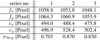
series no. 1 2 3
fx[Pixel] 1058.8 1053.8 1048.1
fy[Pixel] 1064.3 1060.9 1053.9
cx[Pixel] 494.0 488.4 475.8
cy[Pixel] 496.9 528.4 502.4
σRep[Pixel] 0.703 0.870 0.830
Table 1: Optical path calibration results forfL = 12mm. The optical path calibration was performed three times for the12mm focal length. For each calibration series a chessboard pattern was recorded from 50 different perspectives.
to5.2m. For the12mm lens the pattern was recorded at 50 dif-ferent object distancesoin the range from approximately0.7m to3.9m. Since each pattern has 54 reference points, 54 measure-ment points are received for each object distanceo.
To evaluate the three calibration methods different experiments were performed based on the two series of measurements. Beside the physical model and the behavioral model based calibration method, the curve fitting approach was performed by using a third and a sixth order polynomial.
In the first experiment only the values of five measured object distancesowere used for calibration. This experiment was per-formed to evaluate if a low number of calibration points is suffi-cient to receive reliable calibration results.
In a second experiment only the50% of the measurement points with the lowest object distances (forfL = 35mm object dis-tances up to approx.2.6m and forfL= 12mm object distances up to approx.2.1m) were used for calibration. In this experiment it was supposed to investigate how strong the estimated functions are drifting off from the real model outside the range of calibra-tion.
To evaluate the accuracy of the depth map, based on all mea-sured points the root mean square error (RMSE) with respect to the object distance was calculated for both focal lengths. In this experiment the object distances which were calculated from the virtual depth were converted to metric object distance by using the behavioral model presented in Section 3.2.2.
Section 5.2 presents the results corresponding to the experiments performed for the depth map calibration.
5. RESULTS
This section presents the results of the performed experiments. In Section 5.1 the results of the calibration of the optical imaging process are presented, while Section 5.2 shows the results corre-sponding to the calibration of the depth map.
5.1 Calibration of the optical path
As already mentioned in Section 3.1 the used calibration method described in (Zhang, 1999) calculates four intrinsic as well as dis-tortion parameters. The intrinsic parameters are the focal lengths of the underlying pinhole camera (fxandfy) and the correspond-ing principal point (cxandcy). Table 1 and 2 show the calibration results for the12mm and35mm focal length respectively. For both focal lengths the results of the three calibration series are presented in the tables. Besides, for each calibration series the root mean square (RMS) of the reprojection errorσRepwas cal-culated. The reprojection erroreRepis the Euclidean distance be-tween a measured two dimensional (2D) image point and the im-age point which results from the projection of the corresponding
series no. 1 2 3
fx[Pixel] 3259.1 3261.6 3284.0
fy[Pixel] 3262.3 3261.0 3291.0
cx[Pixel] 520.7 430.0 426.3
cy[Pixel] 346.6 389.5 323.6
σRep[Pixel] 0.332 0.333 0.342
Table 2: Optical path calibration results forfL = 35mm. The optical path calibration was performed three times for the35mm focal length. For each calibration series a chessboard pattern was recorded from 50 different perspectives.
three dimensional (3D) object point, based on the camera model. Eq. (32) gives the definition of the RMS of the reporjection error.
σRep= v u u
t1
N ·
N X
i=1
ei Rep
2
(32)
As one can see, the reprojection error for the12mm focal length is about twice to three times as high as the one for the35mm focal length. This can be explained since the effective image res-olution depends on the virtual depth. For a low virtual depth the effective resolution is higher than for a high virtual depth. The
12mm focal length results in a larger field of view (FOV) than the 35mm focal length. Thus, for the12mm focal length the pattern had to be recorded from a much closer distance than for the35mm focal length. This likely resulted in a higher virtual depth. Nevertheless, since the calibration results showed a very high variance between the single calibrations we did not investi-gate this phenomena further.
As one can see from Table 1 and 2, the estimated intrinsic param-eter are varying a lot from one calibration series to the next, es-pecially forfL= 35mm. The reason therefore is that especially for large focal lengths the extrinsic parameter, which have to be estimated for each recorded pattern and the intrinsic parameters are strongly correlated and thus cannot be separated accurately. The calibration could be improved by using a 3D calibration ob-ject. From a 3D object three conditions more than from a planar object are received per perspective.
5.2 Calibration of the depth map
In this section only the results for the calibration of the35mm lens are presented. ForfL = 12mm comparable results were achieved.
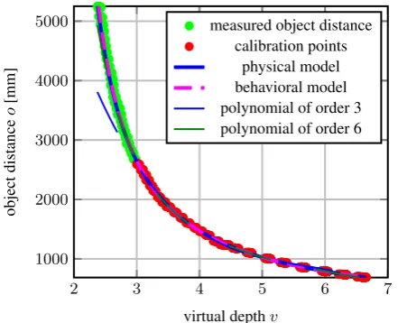
Figure 4 shows the results corresponding to the first experiment. The red dots represent the calibration points for the five object distances. The green dots are the remaining measured points which were not used for calibration. As one can see, the phys-ical model as well as the behavioral model are almost congru-ent. Both curves match the measured distances very well over the whole range from approx. 0.7m to5.2m. For the polynomials of order three and six instead, five object distances are not suf-ficient to approximate the function between virtual depthvand object distanceoaccurately. Both functions fit to the points used for calibration but do not define the underlying model properly in between the calibration points.
2 3 4 5 6 7 1000
2000 3000 4000 5000
virtual depthv
object
distance
o
[mm]
measured object distances calibration points
physical model behavioral model polynomial of order 3 polynomial of order 6
Figure 4: Results of the first experiment for the depth map cal-ibration. Five object distances were used for calcal-ibration. The calibration was performed based on the physical model, the be-havioral model and the curve fitting approach.
2 3 4 5 6 7
1000 2000 3000 4000 5000
virtual depthv
object
distance
o
[mm]
measured object distance calibration points
physical model behavioral model polynomial of order 3 polynomial of order 6
Figure 5: Results of the second experiment for the depth map calibration. Object distances up to approx. 2.6m were used for calibration. The calibration was performed based on the physical model, the behavioral model and the curve fitting approach.
measured distances very well. Nevertheless, for object distances larger than 2.6m especially the third order but also the sixth order polynomial are drifting away from the series of measure-ments. The functions of both model based approaches still match the measured values very well up to an object distance of5.2m. Thus, the functions underlying the two model based calibration methods conform with the reality. Both functions are able to con-vert the virtual depth to an object distance even outside the range of calibration points with good reliability.
As mentioned in Section 4.2, to evaluate the depth resolution of the plenoptic camera the complete series of measurement points was used. For each of the 50 object distances the RMSE is cal-culated. The RMSE is calculated from the 54 valuesoM eas mea-sured for each object distance and the corresponding valueso(v)
calculated as a function of the virtual depthv. The virtual depth valuesvare transformed into object distance based on the func-tion received from the behavioral model. The RMSE is defined
1000 2000 3000 4000 5000
100
101
102
103
object distanceo[mm]
σ
[mm]
fL= 35 mm
fL= 12 mm Rx Spec.fL= 31.98 mm
Figure 6: Depth accuracy of a Raytrix R5 camera with two dif-ferent main lens focal lengths (fL= 35mm andfL= 12mm)
as given in eq. (33).
σ=
v u u
t1
54·
53 X
i=0
o{i}M eas−o(v{i}) 2
(33)
Figure 6 shows the RMSE of the depth for the12mm and the
35mm focal length respectively. Besides, the figure shows the simulated accuracy of the camera which is given by Raytrix. For the simulation a maximum focus distance of 10m and a focal length offL= 31.98mm was defined. Since the RMSE for the
12mm focal length increases strongly with rising object distance, the axis of ordinates is scaled logarithmically.
The results for the focal lengthfL= 35mm conform very well with the specification given by Raytrix. However, it cannot be guaranteed that the object distances measured during the exper-iments are equivalent to the distance given by Raytrix. The dis-tance given by Raytrix is the disdis-tance between an object and the sensor plane. Thus, the Raytrix specification actually might be shifted by a small offset along the axis of abscissas.
As one can see, the accuracy measured forfL= 12mm is worse by a factor of approx. 8 to 10 compared tofL = 35mm. This conforms to the evaluation made in Section 2.2, according to which352
122 = 8.5holds true.
6. CONCLUSION
In this article we developed an analytical expression for the depth map accuracy supplied by a focused plenoptic camera. The ex-pression describes the dependency of the depth accuracy from camera specific parameters like the focal length of the main lens
fL.
Besides, it was shown that the image synthesized from the cam-era’s raw image can be described by the projection model of a pinhole camera. Hence, the intrinsic and distortion parameters of the synthesized image can be estimated by traditional calibration methods.
measurements is needed for calibration. Besides, it was shown that the estimated functions are valid in excess of the calibration range.
In future development the method for calibrating the optical imag-ing process has to be improved since the estimated intrinsic and distortion parameters showed high variances. A reliable estima-tion of the camera parameters is needed to calculate an accurate 3D point cloud from the depth map supplied by the camera.
In near future the plenoptic camera is supposed to operate in nav-igation applications for visually impaired people. The camera seems to be suited for such an applications because of its small dimensions. Furthermore, the depth map accuracy is sufficient for this purposes.
ACKNOWLEDGEMENT
This research is funded by the Federal Ministry of Education and Research of Germany in its program ”IKT 2020 – Research for Innovation”.
REFERENCES
Brown, D. C., 1971. Close-range camera calibration. Photogram-metric Engineering 37(8), pp. 855–866.
Dansereau, D., Pizarro, O. and Williams, S., 2013. Decoding, calibration and rectification for lenselet-based plenoptic cameras. In: IEEE Conference on Computer Vision and Pattern Recogni-tion (CVPR), pp. 1027–1034.
Gortler, S. J., Grzeszczuk, R., Szeliski, R. and Cohen, M. F., 1996. The lumigraph. In: Proceedings of the 23rd annual con-ference on computer graphics and interactive techniques, SIG-GRAPH ’96, ACM, New York, NY, USA, pp. 43–54.
Ives, F. E., 1903. Parallax steregram and process of making same.
Johannsen, O., Heinze, C., Goldluecke, B. and Perwa, C., 2013. On the calibration of focused plenoptic cameras. In: GCPR Workshop on Imaging New Modalities.
Lippmann, G., 1908. Epreuves rversibles. photographies int-grales. Comptes Rendus De l’Acadmie Des Sciences De Paris 146, pp. 446–451.
Lunsdaine, A. and Georgiev, T., 2008. Full resolution lightfield rendering. Technical report, Adobe Systems, Inc.
Ng, R., 2006. Digital light field photography. PhD thesis, Stan-ford University, StanStan-ford, USA.
Perwass, C. and Wietzke, L., 2012. Single lens 3d-camera with extended depth-of-field. In: Human Vision and Electronic Imag-ing XVII, BurlImag-ingame, California, USA.