Vol. 42 (2000) 253–263
Managerial reputation and the ‘endgame’
Peter Berck
1,∗, Jonathan Lipow
2Department of Agricultural and Resource Economics, University of California, 207 Giannini Hall, Berkeley, CA 94720, USA
Received 5 January 1998; received in revised form 31 August 1999; accepted 31 August 1999
Abstract
This paper examines endgame behavior, specifically the behavior of managers whose primary concern is to retain their jobs. Managers are taken to be of two types, good and bad, and only one manager is randomly selected as the firm’s first-period manager. The manager unobservably chooses the mean and standard deviation (limited by a mean-standard deviation frontier) of the process that generates his observable performance. The good manager can choose higher values of the mean of the outcome-generating process, for given standard deviation, than the bad manager can. After the first of the two periods, the firm’s owner must choose to retain or replace her manager based upon performance. In an endgame-perfect Bayesian equilibria of this reputation game, a good manager chooses a strategy with minimal standard deviation for a given mean while a bad manager chooses a strategy of maximal standard deviation for a given mean. Examples of this type of behavior drawn from finance and sports are given in the paper. The perfect Bayesian equilibria of this game also include conservative, reckless, and herd managerial behavior. © 2000 Elsevier Science B.V. All rights reserved.
JEL classification:C72 Keywords:Reputation; Game
1. Introduction
A typical basketball game is characterized by an ever-widening divergence in tactics as the game approaches its conclusion. The team that is leading tends to play cautiously and
∗Corresponding author. Tel.:+1-510-642-7238; fax:+1-510-643-8911.
E-mail address:[email protected] (P. Berck)
1Peter Berck is a Professor of Agricultural and Resource Economics and a Member of the Giannini Foundation of Agricultural Economics, University of California, Berkeley.
2Jonathan Lipow is a Visiting Lecturer in the Department of Agricultural Economics, Hebrew University, Jerusalem.
slow down the game’s pace even under the pressure of the ‘shot clock.’ The trailing team invariably adopts the antithesis of the leading team’s approach. The endgame tactics of trailing teams are dominated by fast breaks and desperate attempts for three-point baskets. It is our belief that the incentives often facing managers concerned with enhancing or protecting their reputations are analogous to those faced in basketball’s endgame. A manager is ‘ahead’ when his performance to date has enhanced his reputation. Such a manager can be expected to avoid taking risks that may endanger his reputation even if these risks are well justified from the owner’s perspective. A manager is ‘behind,’ however, when performance to date has eroded his reputation. Such a manager must restore his reputation or face dismissal. Such managers are likely to take excessive risks in hope of salvaging their reputations. After all, the money being gambled with belongs to someone else and, if nothing is done, unemployment is unavoidable. Hence, there is little to lose.
In this paper, we will present a model in which managers of varying abilities choose strate-gies for their companies while companies only decide whether or not to retain managers. A strategy determines the mean and standard deviation of the company’s performance. Better managers have access to strategies that dominate those of less-capable managers in the sense that better managers can choose strategies with a higher mean for a given standard deviation or lower standard deviation for a given mean. One intuitively appealing perfect Bayesian equilibrium to this game is that the less-capable managers deliberately choose high-standard deviation strategies, exactly like the trailing basketball team, while more capable managers choose low-standard deviation strategies, exactly like the leading basketball team. We call this equilibrium an ‘endgame’ equilibrium.
We believe that the conditions required to induce this equilibrium are often observed in the real world. Managers who are candidates for endgame-type behavior are likely to work for firms where direct observation of managers is costly, leading owners to infer both manager abilities and decisions based on observation of easily-identified benchmarks, such as earnings, sales, or free cash flow. Such conditions are common in firms where (1) ownership is sufficiently dispersed that the costs of monitoring manager decision making is prohibitive for any single or small group of shareholders or (2) the firm is sufficiently small that it has not attracted any objective analytical following among financial firms. Publicly-owned firms that share these characteristics are well represented on all the major stock exchanges.
Endgame incentives arise when a firm must make a judgement to retain an employee. Long-term contracts would then seem to be a way of minimizing this effect. However, long-term contracts are effectively impossible in many industries and situations. The secu-rities industry is the best example. Money flows into and out of mutual funds quite rapidly in response to fund performance. Some funds place penalties on early withdrawal or charge points to limit mobility, but the mobility persists. Consider a fund owner’s incentives. If the owner contracts to retain managers that he would not retain in a world without commit-ment, the owner will lose his customers to new firms that have no such contracts. Since the customers cannot be committed, the firm owner cannot be committed either. It is, just as modeled, first-period performance that determines second-period retention.
ratio. In situations where bankruptcy costs are high, it is even conceivable that the incen-tive for poor managers to take excessive risks may lead to complete extinction of certain classes of firms which, absent the moral hazard of endgame incentives, would have played a productive role in society.
A vivid illustration of endgame behavior among managers is furnished by the tale of a hapless Chilean copper trader. Working the graveyard shift, the trader incorrectly entered a trade and lost a few million dollars for Chile’s national copper firm. Desiring to cover up his embarrassing error, the trader proceeded to engage in a series of futures speculations using the firm’s money. The trader’s original aim was to make good the initial loss before he was reprimanded. After a series of additional losses, the trader’s objective became to make good the losses before he was dismissed. As losses mounted even further, the objective became to make good the losses before being arrested. As this process developed, the level of risk taken by the trader grew ever larger. His losses were finally noticed, and the trader was arrested but only after he had managed to lose US$ 200 million (living proof that individuals can, indeed, have a noticeable impact on national accounts).
Given recent financial debacles, it appears that the monitoring of manager decision mak-ing is particularly costly in financial tradmak-ing and that endgame behavior is rampant in finan-cial firms. Empirical evidence that portfolio managers alter the risk/return characteristics of their investments in order to affect their reputations (as measured by the flow of money into funds that they manage) is provided in Chevalier and Ellison (1995) and Falkenstein (1996).
There are five sections in this paper. In Section 2, we briefly review the research conducted so far on the importance of managerial reputation in influencing firm decision making. In Section 3, we define the basic parameters of a labor market and delineate formal mathe-matical conditions for perfect Bayesian equilibria in that market. In Section 4, we present a class of graphically and algebraically tractable examples that exhibit endgame behavior. In Section 5, we conclude the paper by summarizing and analyzing our results and by discussing the implications of endgame behavior for mechanism design.
2. Literature review
An extreme form of managerial conservatism is the herding behavior described in Scharf-stein and Stein (1990). In their formulation, managers converged on identical strategies in order to assure that they could do no worse than average. While doing better than average carried rewards, these were outweighed by the costs of underperformance. Hence, all man-agers mimicked each other in order to assure that they would have average performance. While herding is clearly a conservative strategy, it does not imply that clients are always exposed to less-than-optimal levels of risk. One of the portfolio mangers quoted by Scharf-stein and Stein recounts that he was well aware of the stock market’s excessive risk in September 1987, but would not lower his exposure to equities since ‘it was too dangerous to do so.’
Huddart (1996) presented a reputational portfolio management model that induced all types of portfolio managers to take excessive risks. In Huddart’s model, one investment security’s risk/return profile stochastically dominated the other. There were two portfo-lio managers. One was better informed than the other and, if he demonstrated this during the first period, he would be rewarded during the second period. The informed portfolio manager would receive a private signal regarding the inferior security that could make it more attractive. If the information was sufficiently favorable, he would overweight the infe-rior security. Although all managers chose their portfolios simultaneously, the uninformed manager’s need to maximize his chance of appearing to be the informed manager would lead him to overweight the inferior security as well even though his information did not justify such a decision. Meanwhile, the informed manager’s desire to maximize his chance of appearing to be informed would lead him to overweight the inferior security to an extent greater than that justified by the superior information that he possessed.
Zwiebel (1995) also addressed managerial conservatism, presenting a model in which managers had two alternative investment projects to choose from. One project-return profile stochastically dominated the other, but the inferior project’s outcome more clearly signaled the manager’s true level of ability. Average managers preferred the inferior investment that clearly signaled that they were average. Exceptionally capable managers chose the superior investment since they were confident that their abilities would be recognized anyway. Poor managers chose the superior investment since they hoped that the noisier signal would mask their true level of ability.
The model that we present in Section 3 can generate equilibria similar to those of Holm-strom (managerial conservatism), Huddart (managerial recklessness), and Scharfstein and Stein (herd behavior). As we will show in Section 4, it can also generate endgame equilibria.
3. A general two-period model
In this model, an owner hires a manager, observes the manager’s performance in the first of the two periods, and then decides whether or not to retain or replace the manager prior to the second period. Managers are of two types, i, which are good, G, or bad, B. In the first period, the owner knows only the population frequency of good managers,PG, and
outcome and infers from it the likelihood that the manager is good. Based on this inference, the owner retains the manager for a second period or replaces him with a new manager hired at random for the second period. The set of realizations ofYthat lead the owner to replace the manager is known asC — the critical region for the owner’s test of the manager’s abilities. While it is natural forCto be of the form that outcomes lower thany∗will result in the owner firing the manager,Ccan have other forms.
3.1. The nature and behavior of managers
A manager hired by the owner will always receive a one-period contract with a fixed and nonnegotiable payment. Managers will always prefer being employed by the owner to their next best alternative. As a result, the employed manager will make choices that maximize his chance of retention. To maximize their chance of retention, managers choseσ — the standard deviation of the process that generates the outcome,y. The mean for a manager of type i choosingσ is given by a mean-standard deviation (m-sd) frontier,µi(σ). The good
agent’s frontier dominates that of the bad agent; for any given standard deviation, the good agent can achieve at least as high a mean as the bad agent. Both agent’s frontiers include a section with the maximum standard deviation achievable for a given mean called the inefficient section of the frontier. Usually ignored, it plays a critical role in what follows. The examples in the paper depend upon normal likelihood, but the equilibrium concept depends only onµandσ being minimal sufficient statistics. One can show that managers do not choose points inferior to the frontier.3
Taking the owner’s critical region as given, the manager will chooseσ (and, therefore,
µi(σ)) to maximize her chance of retention or minimize her chance of being fired. Now, ℓ(y|µi(σ),σ) is the likelihood of outcome,y, for choice,σ, so its integral over outcomes
in the critical region is the chance of being fired. Thus, the best reply to the owner’sCfor agent of type i (G or B) is
σi∗=arg minσ
Z
C
ℓ(y|µi(σ ), σ )dy. (1)
For simplicity, we will assume that the manager hired by the owner for the second period, unable to alter his own prospects, makes choices that maximize the owner’s expected utility. In our examples, we treat the case where utility is linear, so it is expected that income is maximized.
3.2. The behavior of the owner
For a given pair of managers’ choices,σG∗andσB∗, the owner will choose a set,C, that maximizes her expected utility over both periods. Since the owner chooses a manager at random for the first period, her first-period expected utility is
PG
Z
u(y)ℓ(y|µG(σG∗), σG∗)dy+PB
Z
u(y)ℓ(y|µB(σB∗), σB∗)dy, (2)
whereu(y) is the owner’s utility function. This expected first-period utility is completely determined byσG∗ andσB∗— the choices of managers. It does not directly depend on the owner’s choice ofC. With first-period income determined byσG∗andσB∗, which the owner takes as given, the owner maximizes the sum of her first- and second-period income by maximizing her second-period income.
The owner has a higher income with a good manager in the second period. Therefore, an owner replaces the manager when the Bayesian posterior belief (that is, after observing first-period y) that the manager is good is less than the population frequency of good managers. Letθ1be the ratio of the owner’s posterior probability that the agent is good to
her posterior probability that the agent is bad. Definingθ0asPG/PB, the ratio of population
frequencies of good to bad managers, the owner’s rule for firing a manager is: replace the manager ifθ0>θ1.4 By Bayes’ rule,
Therefore, the realizations ofYfor which the manager will be replaced are those for which the ratio of likelihood functions given above is less than 1. The owner’s best reply toσG∗
andσB∗will be
The choice of critical region is independent of the form of the owner’s utility function. With and only with the assumption of costless replacement, the choice ofCis also independent of the frequency of good agents in the population.
3.3. Equilibrium
The set of strategies
C∗, σG∗, σB∗ described above are a perfect Bayesian Nash equilib-rium because each agent makes the best response to the other agent’s strategy, information is inferred from Bayes’ rule, and the owner’s desired strategy in the second period is the same as her desired strategy in the first period. This last point depends upon two facts: (1) the owner’s critical region maximizes her second-period payoff (her payoff in the game beginning in the second period) as well as the sum of her two-period payoffs and (2) the managers make no strategic choice in the second period.5 Thus, with the context of Nash games, the owner could not do better than the perfect Bayesian equilibrium if she could announce a response in the first period and commit to it. An alternative equilibrium concept would be for the owner to be a Stackleberg leader.
4The replacement criteria, when there is a cost to replacing the manager, is given in the working paper version of this paper, which is available from the authors.
4. Four types of equilibria
There are four different types of perfect Bayesian equilibria supported by the model in Section 3 whenYis distributed normally:6 (1) Good managers display conservatism while bad managers display recklessness. This is the equilibrium that we have characterized as endgame behavior, and a graphical and analytic analysis of this case is presented in this section. The remaining types of equilibrium are shown to be possible by numerical examples. (2) Managers of both types display managerial conservatism, choosing strategies with less-than-maximal mean and on the efficient side of their m-sd frontier. (3) Managers of both types display managerial ‘recklessness,’ choosing strategies on the inefficient side of their frontiers. (4) Managers of both types make the same choice and, therefore, display herd behavior.
4.1. Endgame
An example of endgame behavior is given by the assumption of normality and the fol-lowing m-sd frontiers:
µG=bσG−σG2 and µB=σB−σB2. (5)
Assume that the critical region,C, is an interval of the form [–∞,y∗]. Later, it will be
demonstrated that this is, indeed, true for this class of examples. Letting8(·) be the standard normal cumulative distribution function, the likelihood of performancey∗or less is given
by8(z), wherez=(y∗−µ)/σ.
The manager will choose the value ofσthat minimizes the probability of his being fired,
8(z). Since8is a monotonic increasing transformation ofz, choosingσ to minimize8is the same as choosingσ to minimizez. Substituting the values for managers’ means given by Eq. (5), the managers’ choice problems are
σG∗=arg minσGy
∗−bσ
G+σG2 σG
, (6a)
σB∗=arg minσBy
∗−σ
B+σB2 σB
. (6b)
Setting the derivatives of Eqs. (6a) and (6b) equal to 0 and solving forσ∗, we find that both types of managers’ optimal choice is to setσ∗equal to (y∗)1/2. As a result,µ∗
G=b(y∗)1/2−y∗
andµ∗B=(y∗)1/2−y∗. Since both managers choose the same value forσ∗(and two normal
likelihoods with the same standard deviation cross only once), there is only one value ofY,
y∗, where the ratio of likelihood functions is equal to 1 and the critical region is of the form
[–∞,y∗).
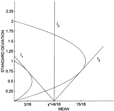
Fig. 1. A graphic example of equilibrium behavior.
From Eq. (4), the owner’s choice ofy∗must be at the point whereℓR/ℓB=1. Setting the
normal likelihood functions for both types of managers equal to one another, substituting (y∗)1/2forσ∗, and simplifying, the equation fory∗is
[b(y∗)1/2−2y∗]2=[(y∗)1/2−2y∗]2. (7) Solving Eq. (7) fory∗, we find thaty∗=(b+1)2/16 andσ∗=(b+1)/4. Substituting this value
ofσ∗ into Eq. (5), we find that the mean for a bad manager is (2b−b2+3)/16 while the mean for a good manager is (6b−b2+7)/16. Evaluated atb=2, the probability that a good manager will be retained is 0.81 while the probability that a bad manager will be retained is 0.19.
Managers’ decision-making process can readily be represented graphically in m-sd space. This equilibrium is illustrated in Fig. 1 for the case ofb=2. The m-sd frontiers for both managers are the curves that start at 0 and end at 1 for the bad manager and 2 for the good manager. The manager is indifferent between those choices ofµandσ for which the probability of being fired is the same. Therefore, the manager’s indifference curves are the combinations ofµandσthat produce the same value ofz,
µ= −zσ+y∗. (8)
In the diagram, these indifference curves are labeled I. All of the indifference curves con-verge at the point whereµ=y∗andσ=0. At this point,zis undefined. From this point, the
indifference curves fan out, with I3preferred to I2 preferred to I1. Managers choose the
of managers have chosen the same level of standard deviation, but good managers have a higher mean than bad managers. Good managers are on the efficient portion of their m-sd frontiers while bad managers are on the inefficient portion of their m-sd frontiers. The bad manager has taken the maximum standard deviation for given mean, which is an example of endgame behavior.
An interesting characteristic of the model is that an increase in the ability of good man-agers has an ambiguous effect on EY over both periods. Assuming thatb=2, and calculating the resulting values for first- and second-period mean returns for both types of managers as well as their probabilities of survival, we find that EY over both periods is equal to 1.53PG+0.44.
Now, let us assume that there is an increase in the ability of good managers so thatb=3. By calculating the resulting values for first- and second-period returns and probabilities of survival, we find that EY over both periods equals 4.17PG+0.08.
Comparing these results, we see that EY’s relationship to the value ofbdepends critically on the value ofPG. IfPG<0.125, then an increase in the ability of good managers from
b=2 tob=3 lowers EY over both periods. IfPG>0.125, then an increase in the ability of good managers fromb=2 tob=3 raises EY over both periods.
The intuition behind this is that increases in the ability of good managers force bad managers into taking ever-more-desperate gambles. This can offset all of the other benefits of the increase in ability. When the value ofbis raised from 2 to 3, the managers’ choice of
σincreases from 3/4 to 1. As a result,µBdeclines from 3/16 to 0 whileµGincreases from
15/16 to 2. The expected second-period return for good managers,µG2, increases from 1 to
2.25 whileµB2is unchanged. The probability that a good manager will be retained following
observation of first-period results increases from 0.81 to 0.84 while the probability of bad managers’ retention falls from 0.19 to 0.16. If bad managers are far more common than good managers, the first-period decline in mean return for them outweighs the first-period gain in mean return for good managers. Since good managers are rare, increases in their second-period mean return or in the probability that good (bad) managers are retained (replaced) hardly matter. Replacing a bad manager is meaningless if his replacement is almost inevitably just as bad a manager.
4.2. Conservatism
Let the m-sd frontiers of the two managers be
µG=2
σG−σG2
and µB=σB−σB2. (9)
The following perfect Bayesian equilibria was found by numerical methods: The owner setsC∗=(–∞, 0.114]∪[0.483,∞). Here,Cis two disjoint intervals. As before, managers
of a bad manager getting rehired is 0.543. The likelihood functions for the two managers are equal whenyis 0.114 and 0.483, completing the equilibrium. The equilibrium shows conservatism since both managers’ (µ,σ) choices are on the efficient portion of their m-sd frontiers. The good manager has chosen a lower level of standard deviation than the bad manager, andµG>µB.
4.3. Herding
Let the frontiers be given by Eq. (5). If both types of manager setµandσequal to 0, the result is herding behavior similar to that of Scharfstein and Stein (1990). In this equilibrium,
C∗=(–∞,−y∗]∪[y∗,∞). Given this critical region, agents will setµandσ equal to 0. If agents do so, the owner will have no reason to alter her choice ofC. The owner is not well served by this equilibrium.
4.4. Reckless
Again, let the m-sd-frontiers be Eq. (5). The owner choosesC∗=(−1.36, 1.36). Both man-agers maximize their probability of being outside ofCby choosing their maximum-attainable standard deviation−σG=2 andσB=1 andµi=0. TheC∗is one of many best responses
to this choice ofσicompleting the equilibrium. In this equilibriumσG>σB,µG>µB, and
no manager is on the efficient portion of his m-sd frontier. The owner is ill served by this equilibrium, and one presumes that a real system would coordinate on one of the first two types of equilibrium.
The herding and reckless examples show that there are multiple equilibria in this model.
5. Conclusion
We have shown how relatively capable managers, influenced by reputational concerns, will behave in a manner that owners regard as overly cautious while less-capable managers, influenced by the same reputational concerns, will behave in a manner that owners regard as overly aggressive. We call equilibria in which such behavior is seen endgame equilibria. Such behavior is likely to take place in a wide variety of real-world managerial settings. In these settings managers unobservably choose investments or business strategies that, combined with their level of ability, generate a stochastic stream of profits. The realization of the profit stream is then used to draw inferences regarding manager ability.
Given that the owner’s interest is in the maximization of profits, the equilibrium behavior described in Section 3 is costly. Bad (good) managers sacrifice mean profits in order to increase (lower) the standard deviation of profits. Furthermore, the equilibrium behavior of managers would not be affected if, rather than profit maximization, owners were interested in maximizing some reasonable utility function. This is because the point where the ratio of likelihood functions equals 1 would remain unchanged regardless of the owner’s utility function. As long as managers choose the same value forσ∗, the owner’s best response,
regardless of their utility functions, remains the same.
This allowed us to greatly simplify the model’s presentation and permitted us to focus on the incongruity between owner and manager preferences. The design of appropriate contractual mechanisms aimed at mitigating endgame-type problems, as well as the influence of such behavior on firms’ decisions regarding capital structure, remains for future research.
In considering the design of contractual mechanisms aimed at mitigating endgame be-havior, it should be appreciated that, unlike standard contingent contracting models, owners attempting to mitigate this type of agency effect may prefer managers to be more, rather than less, risk averse. The reason for this is obvious. In typical contingent contracting, the efficacy of the contract is limited by the degree of manager risk aversion. Owners, assumed to be risk neutral, always wish that managers would be less risk averse and, hence, more willing to accept a share of a stochastic stream of profits. After all, the greater the degree to which manager compensation is tied to profits, the better the alignment of manager and owner preferences.
In the endgame model, however, bad managers behave too aggressively. These managers may not be so willing to sacrifice mean profits in order to increase the standard deviation of profits if they are sharing in those profits. The desire of managers to raise mean income will induce more cautious behavior while the desire to avoid risks will further increase the degree of caution chosen in making decisions regarding the mean and standard deviation of profits. This is exactly what owners want. Hence, depending on the frequency of good and bad managers, owners may see manager risk aversion as facilitating, rather than hindering, the design of contractual mechanisms aimed at reducing the incongruity of preferences between owners and managers.
Acknowledgements
The authors would like to thank Angie Erickson for editorial assistance and an anonymous referee for his insight. The remaining errors are ours.
References
Chevalier, J., Ellison, G., 1995. Risk taking by mutual funds as a response to incentives. Working Paper, University of Chicago.
Falkenstein, E.G., 1996. Preferences for stock characteristics as revealed by open-end mutual fund portfolio holdings. Journal of Finance 51, 111–135.
Fama, E., 1980. Agency problems and the theory of the firm. Journal of Political Economy 88, 288–307. Fudenberg, D., Tirole, J., 1993. Game Theory. MIT Press, Cambridge, MA.
Gibbons, R., Murphy, K.J., 1992. Optimal incentive contracts in the presence of career concerns: theory and evidence. Journal of Political Economy 100, 468–505.
Holmstrom, B., 1982. Managerial incentive problems: a dynamic perspective. Essays in economics and management in honor of Lars Wahlbeck, Swedish School of Economics, Helsinki, Finland.
Holmstrom, B., Ricart i Costa, J., 1986. Managerial incentives and capital management. Quarterly Journal of Economics 101, 835–860.
Huddart, S., 1996. Reputation and performance fee effects on portfolio choices by investment advisors. Journal of Financial Abstracts: Series A, Corporate Finance and Organization Working Paper Series 3.
Ricart i Costa, J.E., 1989. On managerial contracting with asymmetric information. European Economic Review 33, 1805–1829.