Properly Estimating the Liquidity Effect:
Why Accounting for Stationarity and
Outliers is Important
Hany S. Guirguis
The impulse responses of the federal funds rate to innovations in the non-borrowed reserves are re-examined. The rolling responses reveal that, by correcting for the non-stationarity of the data and including the error correcting terms in the VARs, the liquidity effect found by Christiano et al. (1991, 1992, and 1994) is shortened from six to two months. The rolling responses also locate an outlier between the non-borrowed reserves and the funds rate in May 1980. Once the observation of May 1980 is excluded from the samples, the evidence of the liquidity effect becomes much weaker. © 1999 Elsevier Science Inc.
Keywords: Liquidity effect; Stationarity; Outliers JEL classification: C15, E40, E52
I. Introduction
The ability of monetary policy to directly affect interest rates is central to traditional Keynesian theories of the transmission of monetary shocks to the real sector where incomes are formed. The liquidity effect is also a central element in monetarist theory and recent neoclassical models.1 Several studies have provided strong empirical evidence suggesting the disappearance of the liquidity effect. For example, Mishkin (1982), Cornell (1983), Reichenstein (1987), and Leeper (1992) found no evidence of a liquidity effect. The inability to find any empirical support for the liquidity effect has led to the emergence of some studies focusing on narrow monetary aggregates (like non-borrowed reserves) where monetary shocks are more likely to reflect the Fed’s policy rather than its
Department of Economics, State University of New York at Farmingdale, Farmingdale, New York. Address correspondence to: Dr. H. Guirguis, State University of New York, Farmingdale, Department of Economics, Route 110, Farmingdale, NY 11735-1021.
1For more details, see Friedman (1968) and Lucas (1990).
accommodation of the demand for money. These studies have found that the Fed can affect the nominal interest rate through its open market operations. For example, Strongin (1992), Christiano and Eichenbaum (1991, 1992b), and Christiano et al. (1994) showed that the liquidity effect between the non-borrowed reserves and the federal funds rate lasts for six months.
This paper re-examines the existence and the stability of the liquidity effect between the non-borrowed reserves and the federal funds rate over the last thirty-three years, an era characterized by many changes in the Fed’s policy, and in the way the public forms its inflationary expectations.2The statistical approach in this paper uses the concepts of unit roots and cointegration analysis to account for the non-stationarity of the data, and implements the technique of the rolling impulse response functions to examine the sub-sample stability of the liquidity effect.
The first major finding of this paper is that by correcting for the non-stationarity of the data and including the error correction terms in the VARs, the liquidity effect is shortened from six to two months. The second major finding is that by including the observation of May 1980, when credit controls were suddenly relaxed and aggressive expansionary monetary policies were adopted, one overestimates the longevity and the existence of the two-month liquidity effect over the sample periods.
In summary, the results of the paper lead to the conclusion that the existence of the liquidity effect documented by many of the studies focusing on narrow monetary aggre-gates can be attributed to the non-stationarity of the data and the outlier of 1980:5. Therefore, the main findings reported here underscore the ability of the Fed to peg interest rates through unanticipated money growth.
The remainder of this paper is organized as follows. In Section II, I briefly review literature on the liquidity effect. In Section III, I describe and examine the properties of the data. In Section IV, I describe the estimation procedures. In Section V, I discuss the empirical results, and in Section VI, I give my conclusion and summarize the main findings.
II. Literature Review
Traditional economic theories hold that expansionary monetary policy can generate a transitory decline in nominal interest rates. A key element in the transmission from money supply to interest rates is short-run stickiness of prices in the labor and goods market. Therefore, the increase in money supply leads to an increase in real money balances and an excess supply. As the real money supply increases, economic agents become more liquid and adjust their portfolios by buying more bonds. This bids up real bond prices and generates a liquidity effect by decreasing the nominal interest rate.
The increase in bond prices and decrease in the nominal interest rate encourage economic agents to invest their money in non-financial commodities. This increases the general level of income and price, and thus stimulates the demand for money. As a result, the excess supply of monetary assets is reduced due to income and price effects, which leads to a rise in the interest rate. The longer it takes the income and the price effect to overcome the liquidity effect, the more effective is monetary policy in reducing interest rates.
To measure the liquidity effect, many studies have utilized the unrestricted (atheoreti-cal) Vector Autoregressions (VAR) where measures of money, interest rate, income, and prices are included. The setup of the VAR used in this paper is an extension to the ones adopted by Christiano and Eichenbaum (1991) and Gorden and Leeper (1991), where an additional measure of the world commodity prices is included to account for the price puzzle documented by Sims (1992).
III. Data Analysis
Data Description
The variables included in the VARs fall into five categories: non-borrowed reserves (M), industrial production (Y), the consumer price index minus shelter (P), the spot market index for all commodities (CP), and the federal funds rate (N).
Non-borrowed reserves. Estimates for money supply were used to account for the immediate change in interest rate (initial liquidity effect). The rationale for choosing non-borrowed reserves as the measure of the Fed’s monetary policy is that non-borrowed reserves are directly controlled by the Federal Open Market Committee (FOMC). There-fore, innovations in non-borrowed reserves, initiated by the Fed, are more likely to reflect shocks to the money supply rather than to money demand, as in the case of the broader monetary aggregates like M1 and M2.3
Industrial production. Measures of output were included to account for the changes in interest rate caused by the change in the level of economic activities (income effect).
Consumer price index minus shelter. Measures of aggregate price were used to capture the responses of interest rate to the changes in the demand for money (price-level effect).
Spot market index for all commodities. Measures of the spot market index for all commodities (CP) were included to account for the price puzzle, which refers to the negative correlation between inflation and money shocks. Sims (1992) found that the price puzzle can be solved once a proxy for the world commodity prices is included in the VARs to account for the fact that the Fed utilizes this kind of information when setting its reaction function.
Federal funds rate (N). The rationale for using the funds rate as the measure for interest rate was argued by Leeper (1992, p. 4), who stated that:
First, the funds rate is extremely short term, a characteristic that helps separate liquidity effects from expected inflation effects without imposing a theory of the term structure and expected inflation. Second, for data at a monthly frequency, interest rates with maturity structures longer than one month would need to be converted to one month holding period returns. [Leeper (1992, p. 4)]
All the data are from CITIBASE and extend from 1960:01 to 1993:12. In addition, all the variables except for (N) are in logs, and were seasonally adjusted (except for (N) and (CP)).
Stationarity and Cointegration Characteristics of the Data
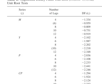
I started my analysis by conducting the Dickey-Fuller test on the level and the growth rate of each variable in the VARs for the whole sample period, extending from 1960:01 to 1993:12. The non-stationarity of the variables has been accounted for by taking the first difference in the case of one unit root, and the second difference in the case of two unit roots. Table 1 displays the results of Dickey-Fuller tests for each variable at 4, 6, 8, 10 and 12 lags, where the lags (K) between brackets are the optimal ones obtained by the procedure advocated by Hall (1990).4The results reveal that at the 5% significance level, M, Y, CP, and N have one unit root. In addition, P has two unit roots in cases of 6, 8, 10, and 12 lags, and one unit root in the case of four lags. The rest of this paper will proceed under the assumption that P has two-unit roots.5
4The procedure advocated by Hall (1990) induces an optimal number of lags greater than or equal the true
order. For more details, see Campbell and Perron (1991).
5Taking the first or the second difference of P had no effect on the responses of N to money innovations. Table 1. Augmented Dickey-Fuller Unit Root (1960:01–1993:12)
Unit Root Tests
* Denotes significance at the 5%; DF:t(z) denotes the Dicky-Fuller t statistics computed using the level of each variable, and DF:t(dz) denotes the Dickey-Fuller t statistics computed using the first difference of each variable.
Next, I formulated the VARs where all the variables are I(0), and the vector error correction model (VECM) where all the variables are I(1). I then tested for the indepen-dent cointegrating vectors among the non-stationary variables in the VECM for the whole sample period. The analysis was conducted using trace tests as specified by Johansen (1988) at 4, 6, 8, 10, and 12 lags. Table 2 suggests there are four different stochastic trends at the 5% significance level and, hence, one independent cointegrating vector.
IV. Estimation Procedure
Model Specification
In line with the initial work of Christiano and Eichenbaum (1991), I specified a baseline VAR which includes the variables in levels as follows:
Model (A)
Mt5constant1Amm~L!Mt1Aym~L!Yt1Apm~L!Pt1Acm~L!CPt1Anm~L!Nt 1em; Table 2. Johansen’s Test on Five-Variable System (1960:01–1993:12)
Number of Lags
Trace
Statistics Null Hypothesis
4 0.6557 There is at least 1
stochastic trend
Estimates of the Error Correction Term (coin):
Coint5(3.957)Mt212(3.341)Yt211(646.278)DPt212(3.464)CPt211
(.166)Nt21.
Yt5constant1Amy~L!Mt1Ayy~L!Yt1Apy~L!Pt1Acy~L!CPt1Any~L!Nt1ey;
Pt5constant1Amp~L!Mt1Ayp~L!Yt1App~L!Pt1Acp~L!CPt1Anp~L!Nt1ep;
CPt5constant1Amc~L!Mt1Ayc~L!Yt1Apc~L!Pt1Acc~L!CPt1Anc~L!Nt1ec;
Nt5constant1Amn~L!Mt1Ayn~L!Yt1Apn~L!Pt1Acn~L!CPt1Ann~L!Nt1en,
where the number of lags is K11 (the equivalent of K lags in difference), and (e) is the orthogonal innovation or the exogenous shock in each equation. The economic rationale for placing m first (M rule) is that innovations in non-borrowed reserves are assumed to be independent of current Y, P, CP, and N. This identification scheme is consistent with Barro (1981), Mishkin (1982), King (1982), Leeper (1992), Strongin (1992), Christiano and Eichenbaum (1991, 1992b) and Christiano et al. (1994).6
To correct for the stationarity of the data, I included the stationary presentation of the variables in the VARs where all the variables are I(0). I also included the one-error correction terms calculated from the whole sample period extending from 1960:01 to 1993:12. The importance of including the error correction terms in the VARs was pointed out by Engle and Granger (1987, p. 259), who stated that:
Thus vector autoregressions estimated with cointegrated data will be mis-specified if the data are differenced, and will have omitted important constraints if the data are used in levels. Of course, these constraints will be satisfied asymptotically but efficiency gains and improved multistep forecasts may be achieved by imposing them. [Engle and Granger (1987, p. 259)]
In all of the VARs, I also included identities to define the growth rate of each variable as the difference between the current and lagged value of its level. The main reason for including these identities in the VARs was to restrict the long-run movements of the growth rate of each variable to follow the long-run movements in its level. In summary, the empirical model used to examine the existence and the stability of the liquidity effect can be stated as follows:
Model (B)
DMt5constant1Amm~L!DMt1Aym~L!DYt1Apm~L!D2Pt1Acm~L!DCPt 1Anm~L!DNt1amcoint1em;
DYt5constant1Amy~L!DMt1Ayy~L!DYt1Apy~L!D2Pt1Acy~L!DCPt
1Any~L!DNt1aycoint1ey;
D2P
t5constant1Amp~L!DMt1Ayp~L!DYt1App~L!D2Pt1Acp~L!DCPt
1Anp~L!DNt1apcoint1ep;
DCPt5constant
1Amc(L)DMt1Ayc(L)DYt1Apc(L)D2Pt1Acc(L)DCPt1Anc(L)DNt1accoint1ec;
6Strongin (1992) and Christiano and Eichenbaum (1991) found that placing Y and P before M and N in the
DNt5constant1Amn~L!DMt1Ayn~L!DYt1Apn~L!D2Pt1Acn~L!DCPt operator, and coin refers to the error correction terms calculated from the characteristic vector corresponding to the canonical correlation in the Johansen (1988) test:
Coint5~3.957!Mt212~3.341!Yt211~646.278!DPt212~3.464!CPt21
1~.166!Nt21.
Estimation Technique
I started my analysis by estimating the impulse response functions of the funds rate to innovations in the non-borrowed reserve, as specified by the baseline Model (A) for the whole sample period, extending from 1960:1 to 1993:12, at one- to twelve-month horizons. I then used the bootstrapping technique to construct 90% confidence intervals for the responses where the number of draws is 100.
To examine the existence and the stability of the liquidity effect over the sample period extending from 1960:1 to 1993:12, I estimated the rolling impulse response functions of the funds rate in Model (B) with a ten-year window.7I began by estimating the responses for the period 1960:1 to 1970:1 at one- to twelve-month horizons. Then, I dropped and added one month at a time to the starting and the ending dates, respectively. I repeated the process to construct the responses until I reached the end of the sample, where the starting and the ending date are 1983:12 and 1993:12, respectively. The main advantage of the rolling window regressions is that the responses are more sensitive to including or excluding observations from the data set, which helps in locating the changes in the causality between money and the interest rate. Finally, to test the sensitivity of my results to the number of lags in the VARs, I ran all the regressions with 4, 6, 8, 10, and 12 lags for each variable.
V. Empirical Results
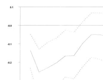
Figure 1 displays the dynamic responses of the funds rate to innovations in the non-borrowed reserves when the variables are in levels. Figure 1 shows that the responses were
7A moving window of shorter than 10 years includes too few observations for reliable results, and windows
significant during the first six months, which is consistent with most of the studies focusing on narrow monetary aggregates, such as non-borrowed reserves.
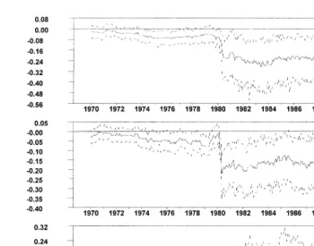
Figures 2 and 3 show the window rolling responses of the funds rate to innovations in the non-borrowed reserves in Model (B) calculated from the VARs with six lags.8As the sample was rolled forward from 1970:1 to 1993:12, the date on the horizontal axis indicates the end date of the ten-year samples. For example, the tests for the sample period extending from 1960:1 to 1970:1 are presented at 1970:1 on the horizontal axis.
Figures 2 and 3 show that the liquidity effect was significant only during the first two months when the data were differenced and the error correction term was included in the VAR. Moreover, Figures 2 and 3 show that the responses of the funds rate in Model (B) were less likely to be significant and important9once the observation of May 1980 was excluded from the regressions. This can be shown by the downward shift in the rolling responses when the observation of 1980:5 was included in the regressions, and the upward shift of the rolling responses at 1990:6 when the observation of 1980:5 was dropped.10
8Because the responses were robust to the different number of lags in the VARs and insignificant at longer
time horizons, I report only the responses calculated from the VARs with six lags at one- to six-month horizons.
9Less important in the sense that the absolute size of the significant responses became smaller.
10To test the robustness of the main results to different sample periods, I estimated forward rolling impulse
The shift in the causality between money innovations and the interest rate in 1980:05 is attributed to the unstable environment created by the sudden changes in the credit control program and the monetary policy during the second quarter of 1980. In the periods preceding 1980:05, the Fed adopted a contractionary monetary policy to fight inflation. On March 14, 1980, the announced program of credit restraint to slow the growth in credit demand confirmed the Fed’s contractionary policy. During the subsequent weeks, the economy experienced a sharp contraction in money measures, and credit growth was well below the FOMC’s specified range. As a result, the real output of goods and services declined markedly in the second quarter of 1980. In the light of these developments, the Board amended the credit program on May 6, 1980, and finally terminated the program on July 3 of that year. In addition, on May 20, 1980, the FOMC adopted expansionary open market operations by increasing the growth rate of non-borrowed reserves by 4%. Most of the additional non-borrowed reserves were used by banks to repay borrowing from the Federal reserve discount window because of the weak demand for money and bank credit. As a result, the federal funds rate declined from 17.61% to 11% (the largest decrease in the funds rate within one month in the last thirty years). This led to the stronger
process to construct the responses until I reached the start of the sample, 1960:1. The results from the forward and backward responses confirmed the main findings of the ten-year moving window.
negative correlation between the federal funds rate and the non-borrowed reserves during May 1980.11
VI. Conclusion and Discussion
In this paper, the important issue of whether the liquidity effect exists was examined for the time period extending from 1960:01 to 1993:12. The empirical model used to evaluate the liquidity effect accounted for both the non-stationarity of the data and the sub-sample instability. The main findings of the paper can be summarized as follows: First, the impulse response functions cast doubt on the validity of estimating the relationship between non-borrowed reserves and the funds rate in levels as specified by Strongin (1992), Christiano and Eichenbaum (1991, 1992b), and Christiano et al. (1994). When I corrected for the non-stationarity of the data and included the error correction terms in the VARs, the responses of the funds rate to money innovations lasted for shorter periods. This result can be attributed to the efficiency loss resulting from not including the cointegration relationship in the VARs, and to a Type I error resulting from not correcting for the non-stationarity of the data.
11For more details, see the Federal Reserve Bulletin from January 1980 to July 1980.
Second, the rolling responses locate a shift in the causality between nonborrowed reserves and the funds rate in May 1980 when the FOMC adopted an expansionary monetary policy in fight recession. Including this observation in the samples strengthened the causality between the federal funds rate and non-borrowed reserves. Once the observation of May 1980 was excluded, the responses were less likely to be significant and important.
Examining the money and interest rate series during the 1980s and the early 1990s shows that increasing or decreasing the growth rate of non-borrowed reserves is no longer capable of changing the funds rate by 6.6%, as happened during 1980:5. For example, decreasing the growth rate of non-borrowed reserves during 1984:7 by 11% increased the funds rate by only .16%, and increasing the growth rate of non-borrowed reserves by 3.5% on 1985:12 decreased the funds rate by only .2%. Given the peculiar characteristics of this era, I believe that 1980:05 is an outlier. In summary, the main conclusion of this paper is that there is no strong evidence to support the liquidity effect once one accounts for the non-stationarity of the data and excludes the outlier of 1980:05 from the sample. There-fore, the findings of the paper are in accord with the view that monetary policy cannot lower interest rates and stimulate spending and employment through the traditional Keynesian channel.
The author acknowledges a debt to Jo Anna Gray, Mark Thoma, and Steven Ongena for their comments. Any remaining errors are those of the author.
References
Barro, R. J. 1981. Unanticipated Money Growth and Economic Activity in the U.S. Money,
Expectations and Business Cycles. New York: Academic Press.
Campbell, J. Y., and Perron, P. April 1991. Pitfalls and opportunities: What macroeconomists should know about unit roots. NBER Working Paper No. 100: 141 200.
Christiano, L. J., and Eichenbaum, M. Nov. 1991. Identification and the liquidity effect of a monetary policy shock. NBER Working Paper No. 3920.
Christiano, L. J., and Eichenbaum, M. May 1992a. Liquidity effects and the monetary transmission mechanism. American-Economic-Review 82:346–353.
Christiano, L. J., and Eichenbaum, M. Aug. 1992b. Liquidity effects, monetary policy, and the business cycle. NBER Working Paper No. 4129.
Christiano, L. J., Eichenbaum, M., and Evans, C. June 1994. The effect of monetary shocks: Evidence from the flow of funds. NBER Working Paper No. 4699.
Cornell, B. Jan. 1983. Money supply announcements and interest rates: Another view. Journal of
Business 56:644–657.
Engle, R. F., and Granger, C. W. J. March 1987. Cointegration and error correction: Representation, estimation, and testing. Econometrica 55:251–276.
Friedman, M. March 1968. The role of monetary policy. American Economic Review 58:1–17. Gordon, D. and E. Leeper. 1991. In search of the Liquidity Effect, Unpublished manuscript, Federal
Reserve Board of Governors.
Johansen, S. Jan. 1988. Statistical analysis of cointegration vectors. Journal of Economic Dynamics
and Control 12:231–254.
King, S. R. 1982. Real interest rates and the interaction of money, output, and prices. Manuscript. Northwestern University.
Leeper, E. M. May/June 1992. Facing up to our ignorance about measuring monetary policy effects.
Economic Review 77:1–16.
Lucas, R. E., Jr. April 1990. Liquidity and interest rates. Journal of Economic Theory 50:237–264. Mishkin, F. S. Feb. 1982. Does anticipated monetary policy matter? An econometric investigation.
Journal of Political Economy 90:22–51.
Reichenstein, W. Jan. 1987. The impact of money on short-term interest rates. Economic Inquiry 25:67–82.
Sims, C. A. Jan. 1992. Interpreting the macroeconomic time series facts: The effect of monetary policy. European Economic Review 36:975–1000.