El e c t ro n ic
Jo ur
n a l o
f P
r o
b a b il i t y
Vol. 14 (2009), Paper no. 62, pages 1827–1862. Journal URL
http://www.math.washington.edu/~ejpecp/
Limit theorems for Parrondo’s paradox
S. N. Ethier
University of Utah Department of Mathematics
155 S. 1400 E., JWB 233 Salt Lake City, UT 84112, USA e-mail:[email protected]
Jiyeon Lee
∗Yeungnam University Department of Statistics 214-1 Daedong, Kyeongsan Kyeongbuk 712-749, South Korea
e-mail:[email protected]
Abstract
That there exist two losing games that can be combined, either by random mixture or by nonran-dom alternation, to form a winning game is known as Parrondo’s paradox. We establish a strong law of large numbers and a central limit theorem for the Parrondo player’s sequence of profits, both in a one-parameter family of capital-dependent games and in a two-parameter family of history-dependent games, with the potentially winning game being either a random mixture or a nonrandom pattern of the two losing games. We derive formulas for the mean and variance parameters of the central limit theorem in nearly all such scenarios; formulas for the mean per-mit an analysis of when the Parrondo effect is present.
Key words:Parrondo’s paradox, Markov chain, strong law of large numbers, central limit theo-rem, strong mixing property, fundamental matrix, spectral representation.
AMS 2000 Subject Classification:Primary 60J10; Secondary: 60F05.
Submitted to EJP on February 18, 2009, final version accepted August 3, 2009.
1
Introduction
The original Parrondo (1996) games can be described as follows: Letp:= 1
2−ǫand
p0:=
1
10−ǫ, p1:= 3
4−ǫ, (1)
where ǫ >0 is a small bias parameter (less than 1/10, of course). In game A, the player tosses a p-coin (i.e.,pis the probability of heads). In gameB, if the player’s current capital is divisible by 3, he tosses ap0-coin, otherwise he tosses ap1-coin. (Assume initial capital is 0 for simplicity.) In both
games, the player wins one unit with heads and loses one unit with tails.
It can be shown that gamesAand B are both losing games, regardless of ǫ, whereas the random mixture C := 1
2A+ 1
2B (toss a fair coin to determine which game to play) is a winning game for
ǫsufficiently small. Furthermore, certain nonrandom patterns, includingAAB,ABB, and AABB but excludingAB, are winning as well, again forǫsufficiently small. These are examples ofParrondo’s paradox.
The terms “losing” and “winning” are meant in an asymptotic sense. More precisely, assume that the game (or mixture or pattern of games) is repeated ad infinitum. LetSn be the player’s cumulative
profit afterngames forn≥1. A game (or mixture or pattern of games) islosingif limn→∞Sn=−∞ a.s., it iswinningif limn→∞Sn =∞a.s., and it is fairif−∞=lim infn→∞Sn <lim supn→∞Sn =∞ a.s. These definitions are due in this context to Key, Kłosek, and Abbott (2006).
Because the games were introduced to help explain the so-called flashing Brownian ratchet (Ajdari and Prost 1992), much of the work on this topic has appeared in the physics literature. Survey articles include Harmer and Abbott (2002), Parrondo and Dinís (2004), Epstein (2007), and Abbott (2009).
GameB can be described ascapital-dependentbecause the coin choice depends on current capital. An alternative gameB, calledhistory-dependent, was introduced by Parrondo, Harmer, and Abbott (2000): Let
p0:= 9
10−ǫ, p1=p2:= 1
4−ǫ, p3:= 7
10−ǫ, (2)
where ǫ > 0 is a small bias parameter. Game Ais as before. In game B, the player tosses a p0 -coin (resp., ap1-coin, a p2-coin, ap3-coin) if his two previous results are loss-loss (resp., loss-win,
win-loss, win-win). He wins one unit with heads and loses one unit with tails.
The conclusions for the history-dependent games are the same as for the capital-dependent ones, except that the patternABneed not be excluded.
Pyke (2003) proved a strong law of large numbers for the Parrondo player’s sequence of profits in the capital-dependent setting. In the present paper we generalize his result and obtain a cen-tral limit theorem as well. We formulate a stochastic model general enough to include both the capital-dependent and the history-dependent games. We also treat separately the case in which the potentially winning game is a random mixture of the two losing games (gameAis played with prob-abilityγ, and gameBis played with probability 1−γ) and the case in which the potentially winning game (or, more precisely, pattern of games) is a nonrandom pattern of the two losing games, specifi-cally the pattern[r,s], denotingrplays of gameAfollowed bysplays of gameB. Finally, we replace (1) by
p0:=
ρ2
1+ρ2 −ǫ, p1:=
whereρ >0; (1) is the special caseρ=1/3. We also replace (2) by
p0:=
1
1+κ−ǫ, p1=p2:= λ
1+λ−ǫ, p3:=1− λ
1+κ−ǫ,
whereκ >0, λ >0, and λ <1+κ; (2) is the special caseκ=1/9 andλ=1/3. The reasons for these parametrizations are explained in Sections 3 and 4.
Section 2 formulates our model and derives an SLLN and a CLT. Section 3 specializes to the capital-dependent games and their random mixtures, showing that the Parrondo effect is present whenever
ρ∈(0, 1) andγ∈(0, 1). Section 4 specializes to the history-dependent games and their random mixtures, showing that the Parrondo effect is present whenever eitherκ < λ <1 orκ > λ >1 and
γ∈(0, 1). Section 5 treats the nonrandom patterns[r,s]and derives an SLLN and a CLT. Section 6 specializes to the capital-dependent games, showing that the Parrondo effect is present whenever
ρ∈(0, 1)andr,s≥1 with one exception: r =s=1. Section 7 specializes to the history-dependent games. Here we expect that the Parrondo effect is present whenever eitherκ < λ <1 orκ > λ >1 and r,s≥1 (without exception), but although we can prove it for certain specific values ofκand
λ(such as κ= 1/9 andλ =1/3), we cannot prove it in general. Finally, Section 8 addresses the question of why Parrondo’s paradox holds.
In nearly all cases we obtain formulas for the mean and variance parameters of the CLT. These parameters can be interpreted as the asymptotic mean per game played and the asymptotic variance per game played of the player’s cumulative profit. Of course, the pattern[r,s]comprisesr+sgames.
Some of the algebra required in what follows is rather formidable, so we have usedMathematica 6 where necessary. Our.nbfiles are available upon request.
2
A general formulation of Parrondo’s games
In some formulations of Parrondo’s games, the player’s cumulative profit Sn after ngames is de-scribed by some type of random walk{Sn}n≥1, and then a Markov chain{Xn}n≥0is defined in terms of{Sn}n≥1; for example, Xn ≡ξ0+Sn(mod 3)in the capital-dependent games, whereξ0 denotes
initial capital. However, it is more logical to introduce the Markov chain {Xn}n≥0 first and then
define the random walk{Sn}n≥1 in terms of{Xn}n≥0.
Consider an irreducible aperiodic Markov chain{Xn}n≥0 with finite state spaceΣ. It evolves accord-ing to the one-step transition matrix1 P= (Pi j)i,j
∈Σ. Let us denote its unique stationary distribution byπ = (πi)i∈Σ. Letw :Σ×Σ 7→Rbe an arbitrary function, which we will sometimes write as a matrix W := (w(i,j))i,j∈Σ and refer to as the payoff matrix. Finally, define the sequences{ξn}n≥1 and{Sn}n≥1by
ξn:=w(Xn−1,Xn), n≥1, (3)
and
Sn:=ξ1+· · ·+ξn, n≥1. (4)
1In the physics literature the one-step transition matrix is often written in transposed form, that is, with column sums
For example, let Σ := {0, 1, 2}, put X0 := ξ0 (mod 3), ξ0 being initial capital, and let the payoff
matrix be given by2
W :=
0 1 −1
−1 0 1
1 −1 0
. (5)
With the role ofPplayed by
PB:=
0 p0 1−p0
1−p1 0 p1
p1 1−p1 0
,
where p0 and p1 are as in (1), Sn represents the player’s profit after n games when playing the
capital-dependent gameB repeatedly. With the role ofP played by
PA:=
0 p 1−p
1−p 0 p
p 1−p 0
,
where p:= 1
2−ǫ, Sn represents the player’s profit afterngames when playing gameArepeatedly.
Finally, with the role ofPplayed byPC :=γPA+(1−γ)PB, where 0< γ <1,Snrepresents the player’s profit afterngames when playing the mixed gameC :=γA+ (1−γ)Brepeatedly. In summary, all three capital-dependent games are described by the same stochastic model with a suitable choice of parameters.
Similarly, the history-dependent games fit into the same framework, as do the “primary” Parrondo games of Cleuren and Van den Broeck (2004).
Thus, our initial goal is to analyze the asymptotic behavior ofSnunder the conditions of the second paragraph of this section. We begin by assuming that X0 has distribution π, so that {Xn}n≥0 and
hence{ξn}n≥1 are stationary sequences, although we will weaken this assumption later.
We claim that the conditions of the stationary, strong mixing central limit theorem apply to{ξn}n≥1.
To say that{ξn}n≥1 has the strong mixing property (or isstrongly mixing) means that α(n)→0 as
n→ ∞, where
α(n):=sup
m
sup
E∈σ(ξ1,...,ξm),F∈σ(ξm+n,ξm+n+1,...)
|P(E∩F)−P(E)P(F)|.
A version of the theorem for bounded sequences (Bradley 2007, Theorem 10.3) suffices here. That version requires thatPn≥1α(n)< ∞. In our setting,{Xn}n≥0 is strongly mixing with a geometric
rate (Billingsley 1995, Example 27.6), hence so is{ξn}n≥1. Sinceξ1,ξ2, . . . are bounded by max|w|,
it follows that
σ2:=Var(ξ1) +2
∞
X
m=1
Cov(ξ1,ξm+1)
converges absolutely. For the theorem to apply, it suffices to assume thatσ2>0.
2Coincidentally, this is the payoff matrix for the classic game stone-scissors-paper. However, Parrondo’s games, as
Let us evaluate the mean and variance parameters of the central limit theorem. First,
µ:=E[ξ1] =
X
i
P(X0=i)E[w(X0,X1)|X0=i] =X
i,j
πiPi jw(i,j) (6)
and
Var(ξ1) =E[ξ21]−(E[ξ1])2=
X
i,j
πiPi jw(i,j)2−
X
i,j
πiPi jw(i,j)
2
.
To evaluate Cov(ξ1,ξm+1), we first find
E[ξ1ξm+1] =
X
i
πiE[w(X0,X1)E[w(Xm,Xm+1)|X0,X1]|X0=i]
=X
i,j
πiPi jw(i,j)E[w(Xm,Xm+1)|X1= j]
= X
i,j,k,l
πiPi jw(i,j)(Pm−1)jkPklw(k,l),
from which it follows that
Cov(ξ1,ξm+1) =
X
i,j,k,l
πiPi jw(i,j)[(Pm−1)jk−πk]Pklw(k,l).
We conclude that
∞
X
m=1
Cov(ξ1,ξm+1) =
X
i,j,k,l
πiPi jw(i,j)(zjk−πk)Pklw(k,l),
whereZ= (zi j)is thefundamental matrixassociated withP(Kemeny and Snell 1960, p. 75).
In more detail, we letΠdenote the square matrix each of whose rows isπ, and we find that ∞
X
m=1
(Pm−1−Π) =I−Π+ ∞
X
n=1
(Pn−Π) =Z−Π,
where
Z:=I+
∞
X
n=1
(Pn−Π) = (I−(P−Π))−1; (7)
for the last equality, see Kemeny and Snell (loc. cit.). Therefore,
σ2=X
i,j
πiPi jw(i,j)2−
X
i,j
πiPi jw(i,j)
2
+2 X
i,j,k,l
πiPi jw(i,j)(zjk−πk)Pklw(k,l). (8)
A referee has pointed out that these formulas can be written more concisely using matrix notation. Denote by P′ (resp., P′′) the matrix whose (i,j)th entry is Pi jw(i,j) (resp., Pi jw(i,j)2), and let 1:= (1, 1, . . . , 1)T. Then
Ifσ2>0, then (Bradley 2007, Proposition 8.3)
lim
n→∞n
−1Var(S
n) =σ2
and the central limit theorem applies, that is, (Sn−nµ)/pnσ2 →d N(0, 1). If we strengthen the
assumption thatPn≥1α(n)<∞by assuming thatα(n) =O(n−(1+δ)), where 0< δ <1, we have (Bradley 2007, proof of Lemma 10.4)
E[(Sn−nµ)4] =O(n3−δ),
hence by the Borel–Cantelli lemma it follows thatSn/n→µ a.s. In other words, the strong law of large numbers applies.
Finally, we claim that, ifµ=0 andσ2>0, then
− ∞=lim inf
n→∞ Sn<lim supn→∞
Sn=∞ a.s. (10)
Indeed, {ξn}n≥1 is stationary and strongly mixing, hence its future tail σ-field is trivial (Bradley
2007, p. 60), in the sense that every event has probability 0 or 1. It follows that P(lim infn→∞Sn= −∞)is 0 or 1. Since µ=0 andσ2>0, we can invoke the central limit theorem to conclude that this probability is 1. Similarly, we get P(lim supn→∞Sn=∞) =1.
Each of these derivations required that the sequence{ξn}n≥1be stationary, an assumption that holds
ifX0 has distributionπ, but in fact the distribution ofX0 can be arbitrary, and{ξn}n≥1 need not be
stationary.
Theorem 1. Letµandσ2 be as in (6) and (8). Under the assumptions of the second paragraph of this
section, but with the distribution of X0 arbitrary,
lim
n→∞n −1E[S
n] =µ and
Sn
n →µ a.s. (11)
and, ifσ2>0,
lim
n→∞n
−1Var(S
n) =σ2 and
Sn−nµ
p
nσ2 →d
N(0, 1). (12)
Ifµ=0andσ2>0, then (10) holds.
Remark. Assume thatσ2>0. It follows that, ifSnis the player’s cumulative profit afterngames for eachn≥1, then the game (or mixture or pattern of games) is losing ifµ <0, winning ifµ >0, and fair ifµ=0. (See Section 1 for the definitions of these three terms.)
Proof. It will suffice to treat the caseX0=i0∈Σ, and then use this case to prove the general case. Let{Xn}n≥0 be a Markov chain inΣwith one-step transition matrixP and initial distributionπ, so
that{ξn}n≥1 is stationary, as above. LetN:=min{n≥0 :Xn=i0}, and define
ˆ
Xn:=XN+n, n≥0.
Then{Xˆn}n≥0is a Markov chain inΣwith one-step transition matrixP and initial stateXˆ0=i0. We
can define{ξˆn}n≥1and{Sˆn}n≥1in terms of it by analogy with (3) and (4). If n≥N, then
ˆ
= ˆξ1+· · ·+ ˆξn−N+ ˆξn−N+1+· · ·+ ˆξn sequences. We also get the last conclusion in a similar way. The first equation in (11) follows from the second using bounded convergence. Finally, the random variableN has finite moments (Durrett 1996, Chapter 5, Exercise 2.5). The first equation in (12) therefore follows from our coupling.
A well-known (Bradley 2007, pp. 36–37) nontrivial example for whichσ2=0 is the case in which Σ⊂Randw(i,j) = j−ifor alli,j∈Σ. ThenSn=Xn−X0 (a telescoping sum) for alln≥1, hence
µ=0 andσ2=0 by Theorem 1.
Substituting in (14) gives
∞
X
m=1
Cov(ξ1,ξm+1) =
X
i,l
πiPilil−
X
i πii2,
and this, together with (13), implies thatσ2=0.
3
Mixtures of capital-dependent games
The Markov chain underlying the capital-dependent Parrondo games has state space Σ ={0, 1, 2} and one-step transition matrix of the form
P:=
0 p0 1−p0
1−p1 0 p1
p2 1−p2 0
, (15)
wherep0,p1,p2∈(0, 1). It is irreducible and aperiodic. The payoff matrixW is as in (5).
It will be convenient below to defineqi:=1−pi fori=0, 1, 2. Now, the unique stationary
distribu-tionπ= (π0,π1,π2)has the form
π0= (1−p1q2)/d, π1= (1−p2q0)/d, π2= (1−p0q1)/d,
whered:=2+p0p1p2+q0q1q2. Further, the fundamental matrixZ= (zi j)is easy to evaluate (e.g.,
z00=π0+ [π1(1+p1) +π2(1+q2)]/d).
We conclude that{ξn}n≥1satisfies the SLLN with
µ=
2
X
i=0
πi(pi−qi)
and the CLT with the sameµand with
σ2=1−µ2+2
2
X
i=0 2
X
k=0
πi[pi(z[i+1],k−πk)−qi(z[i−1],k−πk)](pk−qk),
where[j]∈ {0, 1, 2}satisfies j≡[j](mod 3), at least ifσ2>0.
We now apply these results to the capital-dependent Parrondo games. Although actually much simpler, gameAfits into this framework with one-step transition matrixPAdefined by (15) with
p0=p1=p2:= 1 2−ǫ,
where ǫ > 0 is a small bias parameter. In gameB, it is typically assumed that, ignoring the bias parameter, the one-step transition matrixPB is defined by (15) with
These two constraints determine a one-parameter family of probabilities given by
p1=p2= 1
1+pp0/(1−p0)
. (16)
To eliminate the square root, we reparametrize the probabilities in terms of ρ >0. Restoring the bias parameter, gameBhas one-step transition matrixPBdefined by (15) with
p0:= ρ
2
1+ρ2 −ǫ, p1=p2:=
1
1+ρ−ǫ, (17)
which includes (1) whenρ=1/3. Finally, gameC :=γA+ (1−γ)B is a mixture(0< γ <1)of the two games, hence has one-step transition matrixPC :=γPA+ (1−γ)PB, which can also be defined by (15) with
p0:=γ1
2+ (1−γ)
ρ2
1+ρ2 −ǫ, p1=p2:=γ
1
2+ (1−γ) 1 1+ρ−ǫ.
Let us denote the meanµfor gameAbyµA(ǫ), to emphasize the game as well as its dependence on ǫ. Similarly, we denote the varianceσ2 for gameAbyσ2A(ǫ). Analogous notation applies to games B andC. We obtain, for gameA,µA(ǫ) =−2ǫandσ2
A(ǫ) =1−4ǫ2; for game B,
µB(ǫ) =−
3(1+2ρ+6ρ2+2ρ3+ρ4)
2(1+ρ+ρ2)2 ǫ+O(ǫ 2)
and
σ2B(ǫ) =
3
ρ
1+ρ+ρ2
2
+O(ǫ);
and for gameC,
µC(ǫ) =
3γ(1−γ)(2−γ)(1−ρ)3(1+ρ)
8(1+ρ+ρ2)2+γ(2−γ)(1−ρ)2(1+4ρ+ρ2)+O(ǫ)
and
σ2C(ǫ) =1−µC(0)2−32(1−γ)2(1−ρ3)2[16(1+ρ+ρ2)2(1+4ρ+ρ2)
+8γ(1−ρ)2(1+4ρ+ρ2)2+24γ2(1−ρ)2(1−ρ−6ρ2−ρ3+ρ4)
−γ3(4−γ)(1−ρ)4(7+16ρ+7ρ2)]
/[8(1+ρ+ρ2)2+γ(2−γ)(1−ρ)2(1+4ρ+ρ2)]3+O(ǫ).
One can check thatσ2
C(0)<1 for allρ6=1 andγ∈(0, 1).
The formula forσ2B(0) was found by Percus and Percus (2002) in a different form. We prefer the form given here because it tells us immediately that game Bhas smaller variance than game Afor eachρ 6= 1, provided ǫ is sufficiently small. With ρ = 1/3 and ǫ = 1/200, Harmer and Abbott (2002, Fig. 5) inferred this from a simulation.
The formula forµC(0)was obtained by Berresford and Rockett (2003) in a different form. We prefer
Theorem 2 (Pyke 2003). Letρ >0and let games A and B be as above but with the bias parameter absent. Ifγ∈(0, 1)and C:=γA+ (1−γ)B, thenµC(0)>0for allρ∈(0, 1),µC(0) =0forρ=1,
andµC(0)<0for allρ >1.
Assuming (17) withǫ=0, the conditionρ <1 is equivalent top0< 12.
Clearly, the Parrondo effect appears (with the bias parameter present) if and only ifµC(0)>0. A
reverse Parrondo effect, in which two winning games combine to lose, appears (with anegativebias parameter present) if and only ifµC(0)<0.
Corollary 3 (Pyke 2003). Let games A and B be as above (with the bias parameter present). If
ρ∈(0, 1)andγ∈(0, 1), then there existsǫ0>0, depending onρandγ, such that Parrondo’s paradox
holds for games A, B, and C:=γA+ (1−γ)B, that is,µA(ǫ)<0,µB(ǫ)<0, andµC(ǫ)>0, whenever
0< ǫ < ǫ0.
The theorem and corollary are special cases of results of Pyke. In his formulation, the modulo 3 condition in the definition of gameBis replaced by a modulomcondition, wherem≥3, and game Ais replaced by a game analogous to gameBbut with a different parameterρ0. Pyke’s condition is
equivalent to 0< ρ < ρ0≤1. We have assumedm=3 andρ0=1.
We would like to point out a useful property of game B. We assume ǫ = 0 and we temporarily denote {Xn}n≥0, {ξn}n≥1, and {Sn}n≥1 by {Xn(ρ)}n≥0, {ξn(ρ)}n≥1, and {Sn(ρ)}n≥1 to emphasize
their dependence onρ. Similarly, we temporarily denoteµB(0)andσ2B(0)byµB(ρ, 0)andσ2B(ρ, 0).
Replacing ρ by 1/ρ has the effect of changing the win probabilities p0 = ρ2/(1+ρ2) and p1 = 1/(1+ρ)to the loss probabilities 1−p0and 1−p1, and vice versa. Therefore, givenρ∈(0, 1), we expect that
ξn(1/ρ) =−ξn(ρ), Sn(1/ρ) =−Sn(ρ), n≥1,
a property that is in fact realized by coupling the Markov chains{Xn(ρ)}n≥0 and{Xn(1/ρ)}n≥0 so thatXn(1/ρ)≡ −Xn(ρ) (mod 3)for alln≥1. It follows that
µB(1/ρ, 0) =−µB(ρ, 0) and σ2B(1/ρ, 0) =σ
2
B(ρ, 0). (18)
The same argument gives (18) for gameC. The reader may have noticed that the formulas derived above forµB(0)andσ2B(0), as well as those forµC(0)andσ2C(0), satisfy (18).
Whenρ=1/3, the mean and variance formulas simplify to
µB(ǫ) =−294
169ǫ+O(ǫ
2) and σ2
B(ǫ) =
81
169+O(ǫ)
and, ifγ= 12 as well,
µC(ǫ) =
18
709+O(ǫ) and σ
2
C(ǫ) =
311313105
4
Mixtures of history-dependent games
The Markov chain underlying the history-dependent Parrondo games has state spaceΣ ={0, 1, 2, 3} and one-step transition matrix of the form
P:=
1−p0 p0 0 0
0 0 1−p1 p1
1−p2 p2 0 0
0 0 1−p3 p3
, (19)
where p0,p1,p2,p3 ∈ (0, 1). Think of the states of Σ in binary form: 00, 01, 10, 11. They
rep-resent, respectively, loss-loss, loss-win, win-loss, and win-win for the results of the two preceding games, with the second-listed result being the more recent one. The Markov chain is irreducible and aperiodic. The payoff matrixW is given by
W :=
−1 1 0 0
0 0 −1 1
−1 1 0 0
0 0 −1 1
.
It will be convenient below to define qi := 1−pi for i = 0, 1, 2, 3. Now, the unique stationary
distributionπ= (π0,π1,π2,π3)has the form
π0=q2q3/d, π1=p0q3/d, π2=p0q3/d, π3=p0p1/d,
where d:= p0p1+2p0q3+q2q3. Further, the fundamental matrixZ = (zi j)can be evaluated with some effort (e.g.,z00=π0+ [π1(p1+2q3) +π2(p1p2+p2q3+q3) +π3(p1p2+p2q3+q2+q3)]/d).
We conclude that{ξn}n≥1satisfies the SLLN with
µ=
3
X
i=0
πi(pi−qi)
and the CLT with the sameµand with
σ2=1−µ2+2
3
X
i=0 3
X
k=0
πi[pi(z[2i+1],k−πk)−qi(z[2i],k−πk)](pk−qk),
where[j]∈ {0, 1, 2, 3}satisfies j≡[j](mod 4), at least ifσ2>0.
We now apply these results to the history-dependent Parrondo games. Although actually much simpler, gameAfits into this framework with one-step transition matrixPAdefined by (19) with
p0=p1=p2=p3:= 1 2−ǫ,
where ǫ > 0 is a small bias parameter. In gameB, it is typically assumed that, ignoring the bias parameter, the one-step transition matrixPB is defined by (19) with
These two constraints determine a two-parameter family of probabilities given by
p1=p2 and p3=1−
p0p1
1−p1. (20)
We reparametrize the probabilities in terms ofκ >0 andλ >0 (withλ <1+κ). Restoring the bias parameter, gameB has one-step transition matrixPBdefined by (19) with
p0:=
1
1+κ−ǫ, p1=p2:= λ
1+λ−ǫ, p3:=1− λ
1+κ−ǫ, (21)
which includes (2) when κ = 1/9 and λ = 1/3. Finally, game C := γA+ (1−γ)B is a mixture (0< γ <1) of the two games, hence has one-step transition matrix PC :=γPA+ (1−γ)PB, which also has the form (19).
We obtain, for gameA,µA(ǫ) =−2ǫandσ2A(ǫ) =1−4ǫ
2; for gameB,
µB(ǫ) =−
(1+κ)(1+λ)
2λ ǫ+O(ǫ
2)
and
σ2B(ǫ) = (1+κ)(1+κ+κλ+κλ
2)
λ(1+λ)(2+κ+λ) +O(ǫ); and for gameC,
µC(ǫ) =γ(1−γ)(1+κ)(λ−κ)(1−λ)/[2γ(2−γ) +γ(5−γ)κ
+ (8−9γ+3γ2)λ+γ(1+γ)κ2+4κλ+ (1−γ)(4−γ)λ2
+γ(1+γ)κ2λ+3γ(1−γ)κλ2] +O(ǫ)
and
σ2C(ǫ) =1−µC(0)2+8(1−γ)[2−γ(1−κ)][2λ+γ(1+κ−2λ)]
·[2λ(2+κ+λ)2(1+2κ−2λ+κ2−3λ2+κ2λ−λ3+κ2λ2) +γ(2+κ+λ)(2+5κ−11λ+4κ2−16κλ+2λ2+κ3 −3κ2λ−2κλ2+18λ3+2κ3λ+10κ2λ2−10κλ3+12λ4
+8κ3λ2−8κ2λ3−13κλ4+3λ5+2κ3λ3−6κ2λ4−2κλ5
+κ3λ4+κ2λ5)−γ2(6+14κ−14λ+9κ2−24κλ−9λ2 −18κ2λ+2κλ2+16λ3−κ4−12κ3λ+33κ2λ2+16λ4 −4κ4λ+16κ3λ2+12κ2λ3−30κλ4+6λ5−9κ2λ4−16κλ5
+λ6−4κ4λ3+6κ2λ5−2κλ6−κ4λ4+4κ3λ5+3κ2λ6) +2γ3(1−κλ)2(1+κ−λ−λ2)2]
/{(1+λ)[2γ(2−γ) +γ(5−γ)κ+ (8−9γ+3γ2)λ+γ(1+γ)κ2
+4κλ+ (1−γ)(4−γ)λ2+γ(1+γ)κ2λ+3γ(1−γ)κλ2]3} +O(ǫ).
Theorem 4. Let κ > 0, λ > 0, and λ < 1+κ, and let games A and B be as above but with the bias parameter absent. If γ∈(0, 1) and C := γA+ (1−γ)B, then µC(0)> 0whenever κ < λ <1
or κ > λ > 1, µC(0) = 0 whenever κ= λ or λ = 1, and µC(0) < 0 whenever λ < min(κ, 1) or
λ >max(κ, 1).
Assuming (21) withǫ=0, the conditionκ < λ <1 is equivalent to
p0+p1>1 and p1=p2< 1
2,
whereas the conditionκ > λ >1 is equivalent to
p0+p1<1 and p1=p2>
1 2.
Again, the Parrondo effect is present if and only ifµC(0)>0.
Corollary 5. Let games A and B be as above (with the bias parameter present). If 0< κ < λ <1or
κ > λ >1, and ifγ∈(0, 1), then there existsǫ0 >0, depending onκ,λ, andγ, such that Parrondo’s
paradox holds for games A, B, and C:=γA+ (1−γ)B, that is,µA(ǫ)<0,µB(ǫ)<0, andµC(ǫ)>0,
whenever0< ǫ < ǫ0.
Whenκ=1/9 andλ=1/3, the mean and variance formulas simplify to
µB(ǫ) =−
20
9 ǫ+O(ǫ
2) and σ2
B(ǫ) =
235
198+O(ǫ)
and, ifγ= 1
2 as well,
µC(ǫ) =
5
429+O(ǫ) and σ
2
C(ǫ) =
25324040
26317863+O(ǫ).
Here, in contrast to the capital-dependent games, the variance of game B is greater than that of gameA. This conclusion, however, is parameter dependent.
5
Nonrandom patterns of games
We also want to consider nonrandom patterns of games of the formArBs, in which gameAis played rtimes, then gameBis playedstimes, whererandsare positive integers. Such a pattern is denoted in the literature by[r,s].
Associated with the games are one-step transition matrices for Markov chains in a finite state space Σ, which we will denote by PA and PB, and a function w : Σ×Σ 7→ R. We assume that PA and PB are irreducible and aperiodic, as areP :=Pr
AP s B, P
r−1
A P s
BPA, . . . ,PsBP r
A, . . . ,PBPArP s−1
B (the r+s
cyclic permutations of Pr AP
s
B). Let us denote the unique stationary distribution associated with P
byπ= (πi)i∈Σ. The driving Markov chain{Xn}n≥0 istime-inhomogeneous, with one-step transition
matrices PA,PA, . . . ,PA (r times), PB,PB, . . . ,PB (s times),PA,PA, . . . ,PA (r times), PB,PB, . . . ,PB (s times), and so on. Now define{ξn}n≥1and{Sn}n≥1by (3) and (4). What is the asymptotic behavior
Let us giveX0 distributionπ, at least for now. The time-inhomogeneous Markov chain{Xn}n≥0 is of course not stationary, so we define the (time-homogeneous) Markov chain{Xn}n≥0by
X1 := (X0,X1, . . . ,Xr+s),
X2 := (Xr+s,Xr+s+1, . . . ,X2(r+s)), (22)
X3 := (X2(r+s),X2(r+s)+1, . . . ,X3(r+s)), ..
.
and we note that this is a stationary Markov chain in a subset of Σr+s+1. (The overlap between successive vectors is intentional.) We assume that it is irreducible and aperiodic in that subset, hence it is strongly mixing. Therefore,(ξ1, . . . ,ξr+s),(ξr+s+1, . . . ,ξ2(r+s)),(ξ2(r+s)+1, . . . ,ξ3(r+s)), . . . is itself a stationary, strongly mixing sequence, and we can apply the stationary, strong mixing CLT to the sequence
η1 :=ξ1+· · ·+ξr+s,
η2 :=ξr+s+1+· · ·+ξ2(r+s), (23)
η3 :=ξ2(r+s)+1+· · ·+ξ3(r+s), ..
.
We denote byµˆandσˆ2the mean and variance parameters for this sequence.
The mean and variance parameters µandσ2 for the original sequenceξ
1,ξ2, . . . can be obtained
from these. Indeed,
µ:= lim
n→∞ 1
(r+s)nE[S(r+s)n] =nlim→∞ 1
(r+s)nE[η1+· · ·+ηn] = ˆ
µ
r+s,
whereµˆ:=E[η1], and
σ2:= lim
n→∞ 1
(r+s)nVar(S(r+s)n) =nlim→∞ 1
(r+s)nVar(η1+· · ·+ηn) = ˆ
σ2
r+s,
where
ˆ
σ2:=Var(η1) +2
∞
X
m=1
Cov(η1,ηm+1).
It remains to evaluate these variances and covariances.
First,
µ= 1 r+s
r−1 X
u=0
X
i,j
(πPu
A)i(PA)i jw(i,j) + s−1
X
v=0
X
i,j
(πPr AP
v
B)i(PB)i jw(i,j)
. (24)
This formula forµis equivalent to one found by Kay and Johnson (2003) in the history-dependent setting.
Next,
Πdenoting the square matrix each of whose rows isπ, we can rewrite this as
whereZis the fundamental matrix associated withP:=Pr
APBs. We conclude that
which relies on (25) and (26).
We summarize the results of this section in the following theorem.
Theorem 6. Letµandσ2 be as in (24) and (27). Under the assumptions of the second paragraph of this section, but with the distribution of X0arbitrary,
lim
Remark. It follows that a pattern is losing, winning, or fair according to whetherµ <0, µ >0, or
µ=0.
Proof. The proof is similar to that of Theorem 1, except that N := min{n ≥ 0 : Xn =
In the examples to which we will be applying the above mean and variance formulas, additional sim-plifications will occur becausePAhas a particularly simple form andPBhas a spectral representation. Denote byP′
These assumptions allow us to write (24) as
µ= (r+s)−1πs,rRDsLζ, (28)
and similarly (25) and (26) become
Var(η1) =r+s−
A referee has suggested an alternative approach to the results of this section that has certain ad-vantages. Instead of starting with a time-inhomogeneous Markov chain in Σ, we begin with the (time-homogeneous) Markov chain in the product space ¯Σ:={0, 1, . . . ,r+s−1}×Σwith transition
write the one-step transition matrix in block form as and the central limit theorem. The mean and variance parameters are as in (9) but with bars on the matrices. Of course, ¯Z:= (I−(P¯−Π¯))−1, ¯Πbeing the square matrix each of whose rows is ¯π; ¯P′is as ¯P but withP′
AandPB′ in place ofPAandPB; and similarly for ¯P′′.
The principal advantage of this approach is the simplicity of the formulas for the mean and variance parameters. Another advantage is that patterns other than those of the form[r,s]can be treated just as easily. The only drawback is that, in the context of our two models, the matrices are no longer 3×3 or 4×4 but rather 3(r+s)×3(r+s)and 4(r+s)×4(r+s). In other words, the formulas (28)–(30), although lacking elegance, are more user-friendly.
6
Patterns of capital-dependent games
Let gamesAandBbe as in Section 3; see especially (17). Both games are losing. In this section we show that, for everyρ∈(0, 1), and for every pair of positive integers r andsexcept forr=s=1, the pattern[r,s], which stands for r plays of gameAfollowed bysplays of gameB, is winning for sufficiently smallǫ >0. Notice that it will suffice to treat the caseǫ=0.
We begin by finding a formula forµ[r,s](0), the asymptotic mean per game played of the player’s
ρ >0. First, we can prove by induction that
Pr
and we define the diagonal matrixD:=diag(1,e1,e2). The corresponding right eigenvectors
r2:=
(1+ρ)(1−ρ2+S) 2+ρ+2ρ2+ρ3−ρS
−(1+2ρ+ρ2+2ρ3+S)
,
are linearly independent for allρ >0 (includingρ=1), so we defineR:= (r0,r1,r2)andL:=R−1.
Then
Ps B=RD
sL, s ≥0, which leads to an explicit formula for Ps
BP r
A, from which we can compute its unique stationary
distributionπs,r as a left eigenvector corresponding to the eigenvalue 1. With
ζ:= (2ρ2/(1+ρ2)−1, 2/(1+ρ)−1, 2/(1+ρ)−1)T,
we can use (28) to write
µ[r,s](0) = 1
r+sπs,rRdiag
s, 1−e
s
1
1−e1
, 1−e
s
2
1−e2
Lζ.
Algebraic computations show that this reduces to
µ[r,s](0) =Er,s/Dr,s, (32)
where
Er,s :=3ar{[2+ (3ar−1)(e1s+es2−2es1es2)−(es1+e2s)](1−ρ)(1+ρ)S +ar(es2−e1s)[5(1+ρ)2(1+ρ2)−4ρ2]}(1−ρ)2
and
Dr,s:=4(r+s)[1+ (3ar−1)e1s][1+ (3ar−1)es2](1+ρ+ρ2)2S.
This formula will allow us to determine the sign ofµ[r,s](0)for allr,s, andρ.
Theorem 7. Let games A and B be as in Theorem 2 (with the bias parameter absent). For every pair of positive integers r and s except r=s=1,µ[r,s](0)>0for allρ∈(0, 1),µ[r,s](0) =0forρ=1, and
µ[r,s](0)<0for allρ >1. In addition,µ[1,1](0) =0for allρ >0.
The last assertion of the theorem was known to Pyke (2003). As before, the Parrondo effect appears (with the bias parameter present) if and only ifµ[r,s](0) >0. A reverse Parrondo effect, in which two winning games combine to lose, appears (with anegativebias parameter present) if and only if
µ[r,s](0)<0.
Corollary 8. Let games A and B be as in Corollary 3 (with the bias parameter present). For every
ρ ∈ (0, 1), and for every pair of positive integers r and s except r = s = 1, there exists ǫ0 > 0,
depending onρ, r, and s, such that Parrondo’s paradox holds for games A and B and pattern [r,s], that is,µA(ǫ)<0,µB(ǫ)<0, andµ[r,s](ǫ)>0, whenever0< ǫ < ǫ0.
Proof of theorem. Temporarily denote µ[r,s](0) by µ[r,s](ρ, 0) to emphasize its dependence on ρ. Then, givenρ∈(0, 1), the same argument that led to (18) yields
(This also follows from (32).) It is therefore enough to treat the case ρ ∈ (0, 1). Notice that
On the other hand, if r=s=1, the left side of the last equation becomes
3−1
where the last identity uses the fact that, when s is odd, the odd-numbered bi-nomial coefficients s1
, 3s
, . . . , ss
are equal to the even-numbered ones ss
−1
It follows that, since the caser=1 is excluded,
+ar(e2s−e
Consider next the case in which r ≥1 andsis even. In this case, the last term in (34) is positive, and the remaining terms are greater than 2−(1/4)(5/4)−5/4>0. case we are eliminating a positive contribution, and in the second case we are making a negative contribution more negative. Thus, it will suffice to prove that
2s+2+ [(1+x)s−(1−x)s]−[(1+x)s−(1−x)s](5/x)>0
for 0<x <1, or equivalently that
<−4[4(1/2)−1](1+x)
s−1
(1+x)s−(1−x)s
<−2 (1+x)
s
(1+x)s−(1−x)s <−2,
as required.
Here are four of the simplest cases:
µ[1,1](ǫ) =−
3(1+2ρ+18ρ2+2ρ3+ρ4)
4(1+ρ+ρ2)2 ǫ+O(ǫ 2),
µ[1,2](ǫ) =
(1−ρ)3(1+ρ)(1+2ρ+ρ2+2ρ3+ρ4)
3+12ρ+20ρ2+28ρ3+36ρ4+28ρ5+20ρ6+12ρ7+3ρ8+O(ǫ),
µ[2,1](ǫ) =
(1−ρ)3(1+ρ)
10+20ρ+21ρ2+20ρ3+10ρ4+O(ǫ),
µ[2,2](ǫ) =
3(1−ρ)3(1+ρ)
8(3+6ρ+7ρ2+6ρ3+3ρ4)+O(ǫ).
We turn finally to the evaluation of the asymptotic variance per game played of the player’s cumu-lative profit. We denote this variance byσ[2r,s](ǫ), and we note that it suffices to assume thatǫ=0 to obtain the formula up toO(ǫ).
A formula forσ2[r,s](0) analogous to (32) would be extremely complicated. We therefore consider the matrix formulas of Section 5 to be in final form.
Temporarily denote σ2
[r,s](0) by σ
2
[r,s](ρ, 0) to emphasize its dependence onρ. Then, givenρ ∈ (0, 1), the argument that led to (33) yields
σ2[r,s](1/ρ, 0) =σ[2r,s](ρ, 0), r,s≥1.
For example, we have
σ[21,1](ǫ) =
3ρ
1+ρ+ρ2
2
+O(ǫ),
σ[21,2](ǫ) =3(8+104ρ+606ρ2+2220ρ3+6189ρ4+14524ρ5+29390ρ6
+51904ρ7+81698ρ8+115568ρ9+147156ρ10+169968ρ11
+178506ρ12+169968ρ13+147156ρ14+115568ρ15+81698ρ16
+51904ρ17+29390ρ18+14524ρ19+6189ρ20+2220ρ21
+606ρ22+104ρ23+8ρ24)
/(3+12ρ+20ρ2+28ρ3+36ρ4+28ρ5+20ρ6+12ρ7+3ρ8)3 +O(ǫ),
σ[22,1](ǫ) =3(414+2372ρ+6757ρ2+13584ρ3+21750ρ4+28332ρ5+30729ρ6
/(10+20ρ+21ρ2+20ρ3+10ρ4)3+O(ǫ),
σ[22,2](ǫ) =9(25+288ρ+1396ρ2+4400ρ3+10385ρ4+19452ρ5+29860ρ6
+38364ρ7+41660ρ8+38364ρ9+29860ρ10+19452ρ11
+10385ρ12+4400ρ13+1396ρ14+288ρ15+25ρ16)
/[16(1+ρ+ρ2)2(3+6ρ+7ρ2+6ρ3+3ρ4)3] +O(ǫ).
As functions of ρ ∈(0, 1), σ2
[1,1](0), σ
2
[1,2](0), and σ
2
[2,2](0) are increasing, whereas σ
2
[2,1](0) is decreasing. All approach 1 asρ→1−. Their limits asρ→0+are respectively 0, 8/9, 25/48, and 621/500.
It should be explicitly noted that
µ[1,1](0) =µB(0) and σ2[1,1](0) =σ
2
B(0) (36)
for allρ >0. Since these identities may be counterintuitive, let us derive them in greater detail. We temporarily denote the stationary distributions and fundamental matrices of PB, PAPB, and PBPA, with subscriptsB,AB, andBA, respectively. Then
πB=
1
2(1+ρ+ρ2)(1+ρ
2,ρ(1+ρ), 1+ρ)
and
πBA=
1
2(1+ρ+ρ2)(1+ρ
2, 1+ρ,ρ(1+ρ)),
so
µB(0) =πBζ=0 and µ[1,1](0) = 1
2πBAζ=0. As for the variances, we recall that
σ2B(0) =1+2πBPB′ZBζ=1+πBPB′(2ZBζ)
and
σ[21,1](0) =1+πABPA′(I+PBZABPA)ζ.
ButπABPA′=πBAPBPA′ and
πBPB′ =
1−ρ
2(1+ρ+ρ2)(1+ρ,−ρ,−1),
πBAPBPA′ =
1−ρ
2(1+ρ+ρ2)(1+ρ,−1,−ρ),
2ZBζ= 1−ρ
(1+ρ+ρ2)2
−(1+ρ)(1+4ρ+ρ2) 3+ρ+ρ2+ρ3
1+ρ+ρ2+3ρ3
,
(I+PBZABPA)ζ= 1−ρ
(1+ρ+ρ2)2
−(1+ρ)(1+4ρ+ρ2) 1+ρ+ρ2+3ρ3
3+ρ+ρ2+ρ3
so it follows that
σ2B(0) =σ2[1,1](0) =
3
ρ
1+ρ+ρ2
2
.
An interesting special case of (36) is the caseρ=0. Technically, we have ruled out this case because we want our underlying Markov chain to be irreducible. Nevertheless, the games are well defined. AssumingX0=0, repeated play of gameBleads to the deterministic sequence
(S1,S2,S3, . . .) = (−1, 0,−1, 0,−1, 0, . . .),
hence µB(0) =limn→∞n−1E[Sn] = 0 andσ2B(0) = limn→∞n−1Var(Sn) = 0. On the other hand,
repeated play of patternAB leads to the random sequence
(S1,S2,S3, . . .) = (−1, 0,−1, 0, . . . ,−1, 0, 1, 2, 2±1, 2, 2±1, 2, 2±1, . . .),
where the numberN of initial(−1, 0)pairs is the number of losses at gameAbefore the first win at gameA(in particular,N is nonnegative geometric(12)), and the±1 terms signify independent ran-dom variables that are±1 with probability 12 each and independent ofN. Despite the randomness, the sequence is bounded, so we still haveµ[1,1](0) =0 andσ[21,1](0) =0.
Whenρ=1/3, the mean and variance formulas simplify to
µ[1,1](ǫ) =− 228
169ǫ+O(ǫ
2),
σ2[1,1](ǫ) = 81
169+O(ǫ),
µ[1,2](ǫ) = 2416
35601+O(ǫ), σ
2
[1,2](ǫ) =
14640669052339
15040606062267+O(ǫ),
µ[2,1](ǫ) = 32
1609+O(ǫ), σ
2
[2,1](ǫ) =
4628172105
4165509529+O(ǫ),
µ[2,2](ǫ) = 4
163+O(ǫ), σ
2
[2,2](ǫ) =
1923037543
2195688729+O(ǫ).
Pyke (2003) obtainedµ[2,2](0)≈0.0218363 when ρ=1/3, but that number is inconsistent with Ekhad and Zeilberger’s (2000) calculation, confirmed above, thatµ[2,2](0) =4/163≈0.0245399.
7
Patterns of history-dependent games
Let gamesAandB be as in Section 4; see especially (21). Both games are losing. In this section we attempt to find conditions onκandλsuch that, for every pair of positive integers r ands, the pattern [r,s], which stands for r plays of game Afollowed by s plays of game B, is winning for sufficiently smallǫ >0. Notice that it will suffice to treat the caseǫ=0.
We begin by finding a formula forµ[r,s](0), the asymptotic mean per game played of the player’s cumulative profit for the pattern [r,s], assuming ǫ = 0. Recall that PA is defined by (19) with
p0=p1=p2=p3 := 12, andPBis defined by (19) withp0 :=1/(1+κ), p1=p2:=λ/(1+λ), and
p3:=1−λ/(1+κ), whereκ >0,λ >0, andλ <1+κ. First, it is clear thatPr
A=U for allr ≥2,
As for the spectral representation of PB, its eigenvalues include 1 and the three roots of the cubic
With the help of Cardano’s formula, we find that the nonunit eigenvalues ofPBare
e1 :=
3iare cube roots of unity, and
P:=
Notice that the definitions of P andQ are slightly ambiguous, owing to the nonuniqueness of the cube roots. (If(P,Q) is replaced in the definitions of e1, e2, ande3 by(ωP,ω2Q)or by (ω2P,ωQ),
3Caution should be exercised when evaluatingQnumerically. Specifically, if x<0,Mathematicareturns a complex
root forp3 x. If the real root is desired, one should enter
−p3
1 2
3
4
5
6
0 1 2 3 4 5
0 1 2 3 4 5
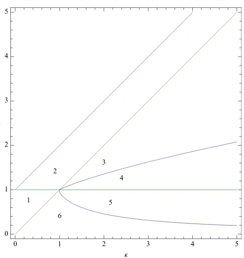
Κ Λ
Figure 1: The parameter space{(κ,λ):κ >0, λ >0, λ <1+κ}, restricted toκ <5 andλ <5. In regions 1, 2, 3, and 6,β2+4α3>0 (e1is real,e2 ande3are complex conjugates); in regions 4 and
5,β2+4α3<0 (e1, e2, ande3 are real). If the conjecture stated below is correct, then, in regions 1, 3, and 4,µ[r,s](0)>0 for allr,s≥1; in regions 2, 5, and 6,µ[r,s](0)<0 for allr,s≥1.
If we define the vector-valued functionr:C7→C4 by
r(x)
:=
−λ(1+κ−λ−λ2)−(1+λ)(1+κ−λ−λ2)x+ (1+κ)(1+λ)2x2 (1+κ−λ−λ2)−(1+κ)(1+λ)(λ−κ)x−(1+κ)2(1+λ)x2
−(1+κ−λ)(1−κλ) + (1+κ)(1−κλ)x
λ(1−κλ)
,
then
r0:= (1, 1, 1, 1)T, r1:=r(e1), r2:=r(e2), r3:=r(e3),
are corresponding right eigenvectors, and they are linearly independent if and only if the eigenvalues are distinct. If the eigenvalues are distinct, we defineR:= (r0,r1,r2,r3)andL:=R−1.
With
u:= 1
4(1, 1, 1, 1) and ζ:=
2/(1+κ)−1 2λ/(1+λ)−1 2λ/(1+λ)−1 2[1−λ/(1+κ)]−1
,
we can use (28) to write
where
Es:=u RDsLζ
with
Ds:=diag
s, 1−e
s
1
1−e1, 1−es2 1−e2,
1−es3 1−e3
.
Algebraic simplification leads to
Es=c0−c1es1−c2es2−c3es3, (39)
where
c0:=
(1+κ)(λ−κ)(1−λ) 4λ(2+κ+λ) ,
and
c1:= f(e1,e2,e3), c2:= f(e2,e3,e1), c3:= f(e3,e1,e2),
with
f(x,y,z):= (λ−κ)[λ(λ−κ)−(1+κ−λ−λ2)x+ (1+κ)(1+λ)x2]
·[1+3κ−2λ+3κ2−4κλ−λ2+κ3−9κλ2+6λ3+2κ3λ −7κ2λ2+6κλ3+κ3λ2−2κ2λ3+4κλ4−2λ5
−(1+κ)(1+λ)(1+2κ−3λ+κ2−2κλ+κ2λ−2κλ2
+2λ3)(y+z) + (1+κ)2(1+λ)2(1+κ−2λ)yz]
/[4(1+κ)3λ(1+λ)2(1−κλ)(1−x)(x−y)(x−z)].
It remains to consider
µ[1,s](0) = (1+s)−1Fs, s≥1, (40)
where
Fs :=πs,1RDsLζ.
Hereπs,1is the stationary distribution ofPBsPA. This is just a left eigenvector of
Rdiag(1,es
1,e
s
2,e
s
3)LPA
corresponding to eigenvalue 1. Writingπˆ= ( ˆπ0,πˆ1,πˆ2,πˆ3):=πs,1, we find that
ˆ
π0 = ˆπ1=
1+f0(e1,e2,e3)e1s+f0(e2,e3,e1)es2+f0(e3,e1,e2)e3s
4+f2(e1,e2,e3)e1s+f2(e2,e3,e1)es2+f2(e3,e1,e2)e3s,
ˆ
π2 = ˆπ3=
1+f1(e1,e2,e3)e1s+f1(e2,e3,e1)es2+f1(e3,e1,e2)e3s
4+f2(e1,e2,e3)e1s+f2(e2,e3,e1)es2+f2(e3,e1,e2)e3s
,
where
f0(x,y,z):= [1+κ−2λ−(1+κ)x]g(y,z)/[2(1+κ)2λ(1+λ)(x−y)(x−z)], f1(x,y,z):= [(1−λ)(1+κ−λ−λ2)−(1+λ)(1−κ2+κλ−λ2)x