Cointegration of Indian Agriculture
with Nonagriculture
Sunil Kanwar, University of Delhi
An oft-repeated refrain in the development literature has been the “neglect” of the agricultural sector vis-a`-vis the industrial sector in the development process of the less developed economies. Because infrastructure is crucially linked to both agricultural and industrial development, poor infrastructure development may make it appear as if slow agricultural growth has caused slow industrial growth. Further, in estimating the relation between agriculture and industry, the former should not be assumed to be exogenous; rather, this should first be established. Moreover, given the presence of nonstationarity conventional regression techniques may yield spurious regressions and significance tests. To circumvent these various problems, we study the cointegration of the different sectors of the Indian economy in a multivariate vector autoregression framework. 2000 Society for Policy Modeling. Published by Elsevier Science Inc.
1. INTRODUCTION
Two roads diverged in a wood, and I— I took the one less traveled by, And that has made all the difference.
Robert Frost
An oft-repeated refrain in the development literature has been the “neglect” of the agricultural sector vis-a`-vis the industrial sector in the development process of the less developed countries. It is argued that with the objective of compressing the growth process into as short a period of time as possible, developing
Address correspondence to S. Kanwar, Department of Economics, Delhi School of Economics, University of Delhi, Delhi 110007, India.
I have benefited from discussions with Ranen Das, K. L. Krishna, Kanchan Chopra, and the seminar participants at the South and Southeast Asian chapter of the Econometric Society meetings held in Delhi in December 1996, and from the incisive comments of the journal referees.
Received February 1997; final draft accepted September 1997.
Journal of Policy Modeling22(5):533–556 (2000)
countries have been trying to industrialize rapidly over the past few decades. The consequence in a bewilderingly large number of countries, if not most, has been the relative neglect of the agricultural sector. This has proved counterproductive for industry itself, as well as for the overall performance of the economy. Indeed, point out the proponents of this view, an overwhelming emphasis on industry appears quite contrary to the perception of even the early development theorists. Although industry was recognized as the “prime mover” in the developing economy, Lewis (1954) realized that “. . . economies in which agriculture is stagnant do not show industrial development” (Timmer, 1988; World Bank, 1982). Extending this argument it is contended that even when agriculture is not stagnant, it must grow in tandem with the other sectors of the economy or else the entire economy-wide growth process may be jeopardized.
development policies tend to stress the leading role of industry. Finally, studies show that most less developed economies have tended to tax their agricultural sectors relative to their industrial sectors by overvaluing their exchange rates, restricting/prohibiting exports of agricultural commodities, and providing sheltered mar-kets to industry. Thus, Rao and Gulati (1994) show that the Aggre-gate Measure of Support1to Indian agriculture works out to2Rs.
196 billion or 22.5 percent of the value of agricultural output for the period 1986–87/88–89. The minus sign implies that Indian agriculture wastaxedto this enormous extent (in contrast to indus-try, which was provided a sheltered market). Viewed in the context of the fact that many LDCs went in for development strategies based on “central planning” that aimed to influence the allocation of resources between agriculture and industry, etc., in accordance with social costs and returns, the above evidence appears to sup-port the thesis of the neglect of the agricultural sector in the development processes of the less developed countries.2This
be-comes an especially important consideration for economies in which the agricultural sector has continued to be very large in terms of national income and employment.
India is a prime example among less developed economies, although hardly an exception, to which the above observations apply. A strategy that placed overwhelming emphasis on the capi-tal-intensive industrial sectors in the economy has left as its conse-quence a feeling of “lost decades” (Bhagwati and Desai, 1979; Lipton, 1968; Eckaus and Parikh, 1968). Further, while agriculture contributed 49 percent of the Gross Domestic Product (at factor cost at 1980–81 prices) in 1950–51, it still contributed as much as 28 percent in 1992–93. By contrast, manufacturing industry grew from about 11 percent to less than 20 percent of GDP over the same period (NAS, various years). The sectoral distribution in terms of shares of employment is even more unequal, with agricul-ture accounting for about 65 percent and manufacturing industry accounting for about 11 percent even as late as 1987–88. In other words, even after 4 decades of planned growth with emphasis on
1The Aggregate Measure of Support is defined as the annual aggregate value of market
price support, nonexempt direct payments and other subsidies not exempt under the reduction commitments under GATT.
2Rao and Caballero [op. cit., p. 904] make the pertinent observation that “The neglect
industry, agriculture continues to be the single largest sector in the economy. The performance of the agricultural sector would then have important implications for the performance of industry. Of course, implicit in this observation is the claim that not only are there important growth linkages between agriculture and industry, but also that the causality runs from the former to the latter. Instead of presupposing this, however, this paper aims to establish the long-run relationship between agriculture and industry in the Indian economy. Stated alternatively, is there a positive, causal relationship between the growth of agriculture and the growth of the industrial sector (as well as the economy) in India?
differentially, it may lead to a significant decline in the relative demand for consumption goods. This, together with the increase in the unit cost of industrial production, would lead to a decrease in industrial profitability, investment and growth (Mitra, 1977). Note, however, that Mitra contended the movement in the terms-of-trade in favor of agriculture to have been brought about by a systematic class bias. Although Chakravarty (1979) concurred with this assessment, Tyagi (1979) did not. In any case, all the studies looking at the terms-of-trade between agriculture and industry including Mitra’s above, use the official wholesale price indices of agricultural and nonagricultural products for this purpose. But, as Ahluwalia observes, what we ideally require is an index of the price of wage goods relative to the price of industrial products. In the absence of such a series, Ahluwalia looks at four alternative series to conclude that the evidence is inconclusive. Further, data do not support the hypothesis of a trend increase in income in-equality in the post-1960s period (see Ahluwalia, 1985, and the references cited therein). Finally, Menon (1986b) reports that for the medium and large public-limited companies (the most important segment of the Indian corporate sector), the post-tax rate of return exceeded the rate of interest for much of the period 1960–61/80–81. And although this margin decreased over time, this was primarily due to an increase in the cost of raw materials and not due to an increase in wage costs. In fact, wage costs as a proportion of the value of production declined over this period (Menon, 1986a). On balance, then, the wage goods constraint does not appear to have tightened over time.
Coming to the role of agriculture as a supplier of raw materials to the agro-industries, Ahluwalia (1985) points out that although there occurred a decline in the rates of growth of output of cash crops in the post-mid-1960s period, this wasnotmatched by de-clines in the growth rates of the corresponding agro-industries. However, we shall not pursue this point further because the avail-able evidence is insufficient to properly address this issue.
is difficult to conclude that if only the growth of agricultural in-comes had been faster, the growth of . . . industries would have picked up. The supply constraints emanating from the infrastruc-turesector, the regulatory framework and poor productivity per-formance would most likely have held back growth . . .” (emphasis added). Note the emphasis we have laid on the infrastructure constraint. We take up this point below.
It is a trite observation that both industrial and agricultural growth are dependent on the availability of adequate infrastruc-ture.3Infrastructure may be thought of as a critical input that itself
does not directly enter production, but which is indispensable to the production activities of the economy. Rao and Caballero (1990, p. 904) note that “. . . without massive investment in . . . roads, extension services, rural education, etc., significant increases in HYV adoption rates or in cropping intensity would not have come about.” Similarly, industrial growth would be retarded by the inadequate availability of power, transport, communications, etc.; as, indeed, Ahluwalia (1985) finds in the case of the Indian econ-omy. Because infrastructure is crucially linked to both agricultural and industrial development, poor infrastructure development by slowing down both agricultural and industrial growth rates may make it appear as if slow agricultural growth has caused slow industrial growth. This has obvious implications in the context of sectoral linkages and policy issues relating to whether the indus-trial sector (“the tail”) should be given overriding emphasis over the agricultural sector (“the dog”), for it calls into question empiri-cal studies that consider the relation between agricultural and industrial growth without properly accounting for the role of the infrastructure “sector.”
Second, empirical studies looking at the relationship between agriculture and industryassumeagriculture to be exogenous, and then estimate the effect it has on the industrial sector (Rangarajan, 1982; Ahluwalia and Rangarajan, 1989). In fact, however, this is a proposition that should be tested first rather than assumed. Third, in specifying the estimable relationships, conventional methods require an a priori bifurcation of the system variables into “endogenous” and “exogenous,” and zero restrictions are sought to be placed on some of these variables to achieve identifi-cation. Although economic intuition may well aid in this regard,
3In this context, by infrastructure we really imply both infrastructure and services. This
such decisions may involve a greater or lesser element of arbitrari-ness and may, hence, be undesirable (Sims, 1980). Fourth, input– output models and multiequation systems have additional draw-backs such as heavy data requirements and untenable assumptions regarding unchanging technology (Rudra, 1967). Fifth, given that most economic time series are trended, conventional regression techniques may yield spurious regressions and significance tests that are uninterpretable (Granger and Newbold, 1986; Phillips, 1986). To circumvent all these problems, we study the cointegra-tion of the various sectors of the Indian economy—namely, agri-culture, manufacturing industry, construction, infrastructure, and services—in a multivariate vector autoregression framework. The basic idea behind such an enquiry is to determine the long-run relationship between these sectors each of which typically exhibits nonstationary behavior. Because economic theory suggests a long-term relationship between (some subset of) these sectors, even though they may appear to be drifting apart over shorter spans of time, over the longer run forces may push them back into equilibrium. If indeed these sectors are moving together along some long-run path, deviations from this path will be stationary. Engle and Granger (1987) formally developed such a cointegrating relationship through the use of an error correction mechanism; which, they suggested, may be estimated by means of a two-step procedure. However, their method assumes the existence of only one cointegration vector, whereas in actual fact there may be more than one error correction mechanism at work in the system. Hence, in this exercise we utilize a more powerful estimation procedure due to Johansen and Juselius (1990, 1992) (and Jo-hansen, 1988), which corrects for this shortcoming through the FIML estimation of a multivariate vector autoregression model. Section 2 briefly sets up the basic model and describes the data used in its estimation. Section 3 presents a discussion of the estima-tion results. Finally, Secestima-tion 4 sketches out the conclusions.
2. BASIC MODEL AND DATA SET
Because economic time series are generally nonstationary pro-cesses, Johansen and Juselius express the unrestricted vector auto-regression model in first differences as:
Dyt5
o
k21
i51 GiDyt2i1 Pyt2k1 mDt1 et, (1)
variables in the system (integrated of order one),Dt is a matrix
of deterministic variables such as an intercept and time trend,et
is NIID (0,V) andGi,P,m,Vare the parameter matrices. Although
the first term in Equation 1 captures the short-run effects on the regressand, the second term captures the long-run impact. Because our objective is to investigate the long-run underlying relation-ships, we focus attention on the elements of matrix II. If the vector yt contains n variables, matrix II will be of order n 3 n, with a
maximum possible rank ofn. Then, using the Granger representa-tion theorem (See Engle and Granger, 1987), if the rank of II is found to ber,n, the matrix II may be factored asab9wherea and b are both of ordern 3r. Matrix b is such thatb9ytis I(0)
even thoughytitself isI(1). In other words, it is the cointegrating
matrix describing the long-run relationships in the model. The weights matrix a gives us the speed of adjustment of specific variables on account of deviations from the long-run relationship.4
We estimate this model for the Indian economy by defining the column vector yt to comprise the (logs of) gross domestic
product at factor cost at constant (1980–81) prices for five sectors: “agriculture,” “manufacturing industry,” “construction,” “infra-structure,” and “services.”5These may be denoted as A, M, C, I,
and S for convenience. Data were available for the period 1950–51/ 1992–93. Preliminary investigation through Dickey-Fuller and Augmented Dickey-Fuller tests revealed the A, I, and S series to be integrated of order 1, whereas M and C were integrated for
4See Hall (1989) for the computation of these constituent matrices.
5These data are taken from the National Accounts Statistics published by the
order 2.6Therefore, the vectory
tis defined as (lnAt,DlnMt,DlnCt,
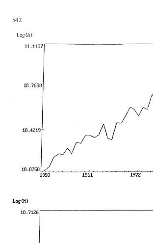
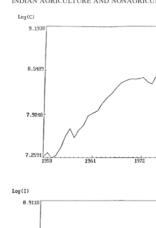
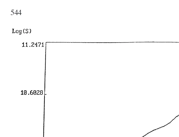
lnIt, lnSt)9. An inspection of the plots of (the logs of) each of the
variables against time supports the inclusion of a time trend (see Figure 1). Hence, a time trend was included both in Equation 1 above as well as in the cointegration space. An important variable that must be predetermined is the maximum lag lengthkin Equa-tion 1 above. Although a long lag may ensure the desired residual properties, it may not make much economic sense regarding ad-justments to deviations from the long-run path (as the bulk of such adjustments are usually found to be completed in a relatively small number of time periods). We foundk52 acceptable on both the above considerations. An inspection of Table 1 (pertaining to the residual statistics from Equation 1 above) supports the assumptions of normality and lack of serial correlation in the error processes of our equation system.7
3. ESTIMATION RESULTS
3A. Testing for the Number of Cointegration Vectors
Several pieces of evidence were adduced to determine the rank of matrix II. First, we use two likelihood ratio tests proposed by Johansen and Juselius (1990, 1992). To test the hypothesis of reduced rank r they propose the use of the trace statistic Qi5
2T Sn
i5r11ln(1 2 li) and maximal eigenvalue statistic Q2 5 2T
ln(12 lr), whereTis the total number of observations andliis
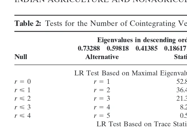
theith eigenvalue. According to both tests (see Table 2), the rank is at least equal to 2. Further, it seems that the rank may well be 3, because both statistics marginally exceed their 95 percent critical values. However, because the computed and critical values of the statistics are virtually the same, we must consider further evidence
6The test results may be had from the author or checked for oneself because the data
are in the public domain. For any variableyithis essentially involves regressingDyton a
constant, trend, andyt21. Lagged terms of the dependent variable may have to be added
to ensure that the error term is white noise. Testing for stationary involves testing whether the coefficient ofyt21is zero, followed by a test for whether the coefficients ofyt21and
the trend are both zero.
7In the case of equations C and S, the Jarque-Bera LM test statistic exceeds the 1 percent
critical value ofx2(2)59.21. However, this may not be serious (also see Johansen and
Figure 1. Continued.
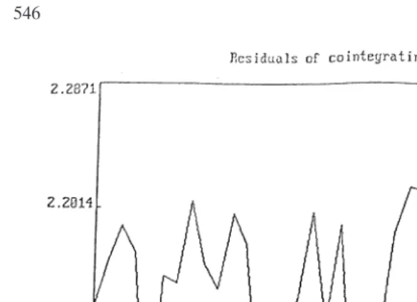
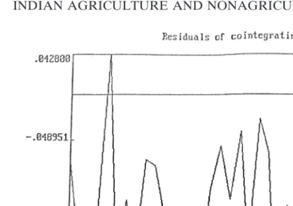
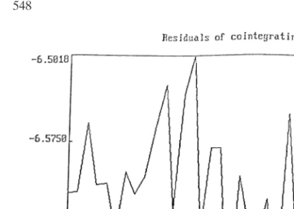
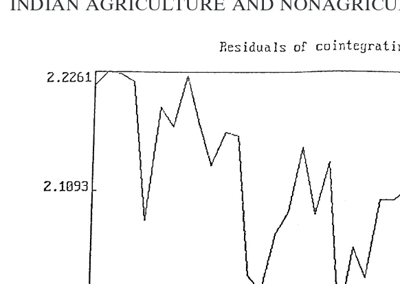
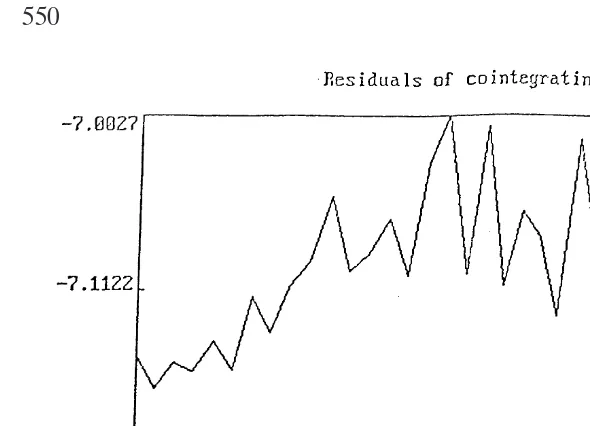
before deciding on the number of cointegrating vectors in this system. Therefore, we next take a look at the graphs of the (residu-als of the) cointegrating relations, and the (residu(residu-als of the) cointe-grating relations corrected for short-run dynamics (Figure 2). If r53 the first three processes must look stationary, whereas ifr5 2, this should hold only for the first two processes. An inspection of Figure 2 suggests thatr 52 would be a more reliable inference, because the graph of the residuals of the cointegrating vector
Table 1: Residuals’ Statistics
Excess Normality AC
Equation Mean SD Skewness kurtosis test coeff.
A 0.000 0.043 20.740 0.509 3.532 0.227
M 0.000 0.029 20.270 1.131 1.650 21.283 C 0.000 0.047 21.049 2.220 12.223 21.817
I 0.000 0.018 0.685 1.654 5.748 0.466
S 0.000 0.012 20.982 2.245 11.519 20.147
Notes:The normality test uses the Jarque-Bera LM statistic, which is distributed as x2(2) under the null. The “AC coeff.” or autocorrelation coefficient refers to the coefficient
Table 2: Tests for the Number of Cointegrating Vectors
Eigenvalues in descending order: 0.73288 0.59818 0.41385 0.18617 0.01334
Null Alternative Statistic 95% c.v.
LR Test Based on Maximal Eigenvalue Statistic
r50 r51 52.8021 33.4610
r<1 r52 36.4704 27.0670
r<2 r53 21.3669 20.9670
r<3 r54 8.2400 14.0690
r<4 r55 0.5370 3.7620
LR Test Based on Trace Statistic
r50 r51 119.4164 68.5240
r<1 r52 66.6143 47.2100
r<2 r53 30.1439 29.6800
r<3 r54 8.7770 15.4100
r<4 r55 0.5370 3.7620
Eigenvalues of the Companion matrix in descending order:
1.00 0.80 0.80 0.27 0.27 0.15 0.15 20.26 20.26 0.03
Notes: The critical values are from Osterwald-Lenum (1992).
corrected for short-run dynamics for the third process appears to show some nonstationarity. Finally, we consider the eigenvalues of the companion matrix (given at the bottom of Table 2).8Because
these eigenvalues give us the reciprocals of the roots of the charac-teristic polynomial, they should lie on or inside the unit circle under the assumption of a cointegrated VAR model. The number of elements equal to or close to unity then give us the number of common stochastic trends in the model. We find that three of the elements are equal to or quite close to one, supporting a choice ofr52. Therefore, we chooser52. The presence of these (two) cointegrating relations in our system reflects an inherent tendency in the system to revert towards equilibrium subsequent to a short-run shock. Thus, the graphs of the cointegrating relations describe
8The companion matrix is given by:
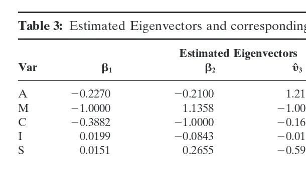
Table 3: Estimated Eigenvectors and corresponding Adjustment Matrix
Estimated Eigenvectors
Var b1 b2 yˆ3 yˆ4 yˆ5
A 20.2270 20.2100 1.2114 20.5618 0.3629 M 21.0000 1.1358 21.0000 21.0000 21.0000 C 20.3882 21.0000 20.1685 20.2610 0.0738 I 0.0199 20.0843 20.0108 0.0172 20.4921
S 0.0151 0.2655 20.5946 0.3721 0.6810
Estimated Adjustment Matrix
Eq. aˆ1 aˆ2 vˆ3 vˆ4 vˆ5
DA 0.0924 (1.26) 0.0241 (0.30) 20.1607 20.0910 20.0095 D2M 0.1545 (7.58) 20.0913 (7.93) 0.0022 20.0524 20.0120 D2C 0.2034 (3.55) 0.2954 (14.6) 0.0218 20.0255 20.0129 DI 0.0363 (0.27) 0.0095 (1.98) 20.0288 0.0278 0.0109 DS 20.0262 (0.02) 0.0070 (1.51) 20.0071 20.0178 20.0086
Notes:Individual components of the LR test statistic for the nullHo:aij50,j51,2
are reported within parentheses.
the deviations from the long-run equilibrium path of the economy on account of the short-run shocks (small or large). And the graphs of the cointegrating relations corrected for these short-run dynamics describe the actual adjustment path correcting for these short-run dynamics. Even though the economy does not stay in equilibrium for any length of time on account of the periodic short-run shocks that it receives, the large number of crossings of the “mean line” displayed in these graphs shows the system’s tendency to return to equilibrium.
3B. The Unrestricted Cointegration Space
In all of the following analysis we assume the presence of two stationary or cointegrating relations and three common stochastic trends in our system. Their estimates are presented in Table 3 along with the corresponding adjustment matrix a. To facilitate the analysis of the cointegration space as summarized by the esti-mates, we also compute certain likelihood ratio test statistics that indicate the relative importance of the individualbandavalues. A test of the null hypothesis fora,Ho:ai15 ai250 tests whether
the equation Dyi contains any cointegrating relation. Individual
3. The estimates tell us that the first eigenvectorb1primarily links
manufacturing sector income positively with agricultural income9
and negatively with construction sector income. The correspond-ing loadcorrespond-ing vectora1and the associated test statistics within
brack-ets tell us that this relation is mostly important in the manufactur-ing and construction sector equations. Note that this vector also reflects the slow “speed of adjustment” of the other variables (i.e., I and S) to the short-run shocks that dislodge the system from its long-run path. Although this implies that we can standardize this eigenvector on either manufacturing sector income or construction sector income, we have chosen to do so on the former. The second eigenvector b2 seems to explain construction sector income as
significantly related to all the variables, with the possible exception of infrastructure sector income. The corresponding weights vector a2indicates that this relation is relatively important in the
construc-tion sector equaconstruc-tion. Therefore, we standardize this eigenvector on the construction variable. Tests for exogeneity (i.e., the joint testHo:aij50, j51,2) strongly support the weak exogeneity of
the agriculture, infrastructure, and services variables. Specifically, for agriculture the test statistic x2(2) 5 1.57, for infrastructure
2.25 and for services 1.53 with p-values of 0.46, 0.32, and 0.47 respectively. This implies that the system may be effectively re-duced to a two-dimensional one without affecting the estimates of b. Alternatively stated, the cointegration relations are to be found in the M and C sector equations only.
We further test for the block exogeneity of the agriculture, infrastructure and services sectors by conducting Granger causal-ity tests. Because our variables are cointegrated, this could be done subject to the cointegration rank and cointegrating vectors. However, Dolado and Lutkepohl (1994) caution that such a proce-dure typically has unknown properties making inferences ques-tionable. Instead, they suggest a simple solution. They point out that the nonstandard asymptotic properties of standard tests on the coefficients of a cointegrated VAR arise from the singularity of the asymptotic distributions of the relevant estimators. They show that this singularity may be removed by estimating a VAR whose order exceeds the “true” order, enabling the use of standard tests. Although they demonstrate the procedure with a Wald test,
9Note that a negative relation betweenDlnM
t(5lnMt/Mt21) and lnAtis consistent with
a positive relation between lnMt and lnAt. This can be easily proved by a numerical
we use the likelihood ratio test below. We first estimate a VAR by regressingytonyt21,yt22, andyt23(i.e., augmenting the “true”
lag order by one fromk52 tok53). We then test for the null hypothesis that the lags of the M and C sector variables do not enter the equations for the A, I, and S sector variables (i.e., the agriculture, infrastructure, and services sectors are block exoge-nous). The likelihood ratio statistic is found to be 20.898, which is distributed asx2with 18 dof and has ap-value of 0.285. Thus,
we cannot reject the null hypothesis of the exogeneity of the agriculture, infrastructure and services sectors vis-a`-vis the manu-facturing and construction sectors of the Indian economy.
4. IMPLICATIONS AND CONCLUSIONS
We now summarize the above results. First, we find that the different sectors of the economy moved together over the sample period and, hence, their development was interdependent. This is not to imply that some of the sectors did not outpace the others, but only that the economic forces at work functioned in such a way as to tie together these sectors in a long-run structural equilibrium. And while short-run shocks may have led to devia-tions from this long-run path, forces existed whereby the system reverted back to it. The significance of this result may be gauged by comparing it to the existence, say, of a positive relationship between the raw data series. Thus, if we were to find a positive relationship between the sectoral incomes in the context of con-ventional econometric models, this could merely be due to the presence of common trends (and not cointegrating relations) in the data and, hence, may not signify a genuine long-run relationship between the growth processes of the different sectors. Although we do find the presence of three common stochastic trends in our data, we also find the presence of two cointegrating relations. In this sense there exists a long-run equilibrium relationship between the different sectors of the Indian economy.
Third, the infrastructure and services sectors (and to a lesser extent the agriculture sector also) exhibit very slow speeds of adjustment to deviations from the long-run path. This is probably reflective of the widespread administrative controls over the activi-ties comprising these sectors for the bulk of the sample period. Thus, the infrastructure subsectors such as electricity, gas, water supply, and communications, and the services subsectors such as rail transport, financial, and insurance services were almost totally within the state sphere over the sample period.10These activities,
therefore, tended to depend on budgetary allocations rather than directly on impulses emanating from the other growing sectors of the economy. This probably undermined the adjustment speeds of these sectors consequent to deviations of the system from the long-run equilibrium path.
Finally, the agriculture, infrastructure and services variables are found to be weakly exogenous with respect to the long-run parameters b. Further, Granger causality tests in the context of cointegrated systems reveal the block exogeneity of these sectors. Note that this exogeneity is notassumedas in some studies noted above. This evidence may be taken to imply that while the agricul-ture, infrastrucagricul-ture, and services sectors significantly affect the process of income generation in the manufacturing and construc-tion sectors, the reverse has not been true. This may be explained by the fact that the growth process in the agricultural sector has important implications for the manufacturing sector11 as we
dis-cussed above. Thus, it relaxes the wage goods, raw material, and foreign exchange constraints and provides a potentially large mar-ket for manufactured products, especially consumer goods. On the contrary, the growth process in the manufacturing sector does not significantly impact the agricultural sector in view of the fact that the predominant bulk of the rural households are either relatively small farmers with small operational holdings and tiny surpluses, or else landless laborers. Given that agriculture is even
10Financial and insurance services came within the purview of the state sector (although
the former not totally) only since the 1960s.
11See also Rangarajan (1982) and Ahluwalia and Rangarajan (1989); although they
today the single largest sector in the economy, it may be seen as a driving force for the other sectors. Similarly, infrastructure development as well as the development of services significantly influence the development of the manufacturing and construction sectors of the Indian economy. Because the reverse linkages to-ward income generation in the infrastructure and service sectors have been found to be weak, encouraging the manufacturing sector alone or even primarily (as in the recent “liberalization” policies) will not help to boost the entire economy in the long run. Rather, the agriculture, infrastructure, and services sectors will have to be directly encouraged.
REFERENCES
Ahluwalia, I.J. (1985)Industrial Growth In India: Stagnation Since the mid-sixties.Delhi: Oxford University Press.
Ahluwalia, I.J., and Rangarajan, C. (1989) A Study of Linkages between Agriculture and Industry: The Indian Experience. InThe Balance between Industry and Agriculture in Economic Development, vol. 2 (Sector Proportions).J.G. Williamson, and V.R. Panchamukhi, (Eds.) New York: Macmillan Press.
Alagh, Y.K., and Sharma, P.S. (1980) Growth of Crop Production: 1960–61 to 1978–79—Is it Decelerating?Indian Journal of Agricultural Economics35:104–118.
Bhagwati, J.N., and Desai, P. (1979)India: Planning For Industrialisation.Delhi: Oxford University Press.
Chakravarty, S. (1974) Some Reflections on the Growth Process in the Indian Economy, Adminstrative Staff College of India, reprinted 1977 inProblems of India’s Eco-nomic Policy.(Wadhwa, C.D., Ed.) Delhi: McGraw Hill.
Chakravarty, S. (1979) On the Question of Home Market and Prospects for Indian Growth.
Economic and Political Weekly14:1229–1242.
Dolado, J.J., and Lutkepohl, H. (1994)Making Wald Tests Work For Cointegrated VAR Systems, mimeo. Germany: Humbolt University.
Eckaus, R.S., and Parikh, K. (1968)Planning for Growth. Cambridge, M.I.T. Press. Engle, R.F., and Granger, C. (1987) Cointegration and Error Correction: Representation,
Estimation and Testing.Econometrica55:251–276.
Granger, C.W.J., and Newbold, P. (1986)Forecasting Economic Time Series, 2nd ed. Orlando, FL: Academic Press Inc.
Hall, S.G. (1989) Maximum Likelihood Estimation of Cointegration Vectors: An Example of the Johansen Procedure.Oxford Bulletin of Economics and Statistics51:213–219. Johansen, S. (1988) Statistical Analysis of Cointegrating Vectors.Journal of Economic
Dynamics and Control12:231–254.
Johansen, S., and Juselius, K. (1992) Testing structural hypotheses in a multivariate cointe-gration analysis of the PPP and the UIP for UK.Journal of Econometrics53:211–244. Johansen, S., and Juselius, K. (1990) Maximum Likelihood Estimation and Inference on Cointegration—With Applications to the Demand for Money.Oxford Bulletin for Economics and Statistics52:169–210.
Krishna, R. (1982) Some Aspects of Agricultural Growth, Price Policy and Equity in Developing Countries.Food Research Institute Studies18:219–260.
Lewis, W. (1954) Economic Development with Unlimited Supplies of Labour.Manchester School of Economic and Social Studies22:139–191.
Lipton, M. (1968) Strategy for Agriculture: Urban Bias and Rural Poverty. InThe Crisis of Indian PlanningP. Streeten, and M. Lipton, Eds. New York: Oxford University Press.
Menon, K.A. (1986a) Interest Cost in Indian Industries: An Econometric Analysis. Eco-nomic and Political Weekly21:837–841.
Menon, K.A. (1986b) Interest Cost and the Rate of Profit in the Indian Corporate Sector.
Economic and Political Weekly21:M44–M51.
Mitra, A. (1977)Terms of Trade and Class Relations.London: Frank Cass.
Mody, A. (1982) Growth, Distribution and the Evolution of Agricultural Markets—Some Hypotheses.Economic and Political Weekly17:25–38.
NAS,National Accounts Statistics, Central Statistical Organisation, Department of Statis-tics, Ministry of Planning, Government of India, various years.
Osterwald-Lenum, M. (1992) A note with quantiles of the asymptotic distribution of the maximum likelihood cointegration rank test statistics.Oxford Bulletin of Economics and Statistics54:461–472.
Phillips, P.C.B. (1986) Understanding spurious regressions in econometrics.Journal of Econometrics33:311–340.
Rangarajan, C. (1982)Agricultural Growth and Industrial Performance in India.Research Report No. 33, International Food Policy Research Institute, Washington, DC. Rao, C.H.H., and Gulati, A. (1994) Indian Agriculture: Emerging Perspective and Policy
Issues.Economic and Political Weekly29:A158–A169.
Rao, J.M., and Caballero, J. (1990) Agricultural Performance and Development Strategy: Retrospect and Prospect.World Development18:899–913.
Rudra, A. (1967)Relative Rates of Growth—Agriculture and Industry. Bombay: University of Bombay.
Sawant, S.D. (1983) Investigation of the Hypothesis of Deceleration in Indian Agriculture.
Indian Journal of Agricultural Economics38:475–496.
Sims, C.A. (1980) Macroeconomics and reality.Econometrica48:1–48.
Srinivasan, T.N. (1979) Trends in Agriculture in India.Economic and Political Weekly
14:1283–1294.
Sundaram, K., and Tendulkar, S.D. (1995)Statistical Tables Relating to the Indian Economy, mimeo. Department of Economics, Delhi School of Economics.
Timmer, C.P. (1988) The Agricultural Transformation. InHandbook of Development EconomicsH. Chenery and T.N. Srinivasan, Eds. Amsterdam: North Holland. Thamarajakshi, R. (1977) Role of Price Incentives in Stimulating Agricultural Production
in a Developing Economy. InGood Enough or Starvation for MillionsD. Ensminger, Ed. Rome: Food and Agriculture Organisation.
Tyagi, D.S. (1979) Farm Prices and Class Bias in India.Economic and Political Weekly
14:A111–A124.