SPECTRAL GRAPH THEORY AND THE INVERSE EIGENVALUE
PROBLEM OF A GRAPH∗
LESLIE HOGBEN†
Abstract. Spectral Graph Theory is the study of the spectra of certain matrices defined from a given graph, including the adjacency matrix, the Laplacian matrix and other related matrices. Graph spectra have been studied extensively for more than fifty years. In the last fifteen years, interest has developed in the study of generalized Laplacian matrices of a graph, that is, real symmetric matrices with negative off-diagonal entries in the positions described by the edges of the graph (and zero in every other off-diagonal position).
The set of all real symmetric matrices having nonzero off-diagonal entries exactly where the graph
Ghas edges is denoted byS(G). Given a graphG, the problem of characterizing the possible spectra ofB, such thatB∈ S(G), has been referred to as the Inverse Eigenvalue Problem of a Graph. In the last fifteen years a number of papers on this problem have appeared, primarily concerning trees. The adjacency matrix and Laplacian matrix ofGand their normalized forms are all inS(G). Recent work on generalized Laplacians and Colin de Verdi`ere matrices is bringing the two areas closer together. This paper surveys results in Spectral Graph Theory and the Inverse Eigenvalue Problem of a Graph, examines the connections between these problems, and presents some new results on construction of a matrix of minimum rank for a given graph having a special form such as a 0,1-matrix or a generalized Laplacian.
Key words.Spectral Graph Theory, Minimum Rank, Generalized Laplacian, Inverse Eigenvalue Problem, Colin de Verdi`ere matrix.
AMS subject classifications.05C50, 15A18.
1. Spectral Graph Theory. Spectral Graph Theory has traditionally used the spectra of specific matrices associated with the graph, such as the adjacency matrix, the Laplacian matrix, or their normalized forms, to provide information about the graph. For certain families of graphs it is possible to characterize a graph by the spectrum (of one of these matrices). More generally, this is not possible, but useful information about the graph can be obtained from the spectra of these various matrices. There are also important applications to other fields such as chemistry. Here we present only a very brief introduction to this extensive subject. The reader is referred to several books, such as [10], [9], [11], [6], for a more thorough discussion and lists of references to original papers.
We begin by defining terminology and introducing notation. Throughout this discussion, all matrices will be real and symmetric. Theordered spectrum(the list of eigenvalues, repeated according to multiplicity in nondecreasing order) of an n×n matrixB will be denote denotedσ(B) = (β1, . . . , βn) withβ1≤. . .≤βn.
AgraphGmeans a simple undirected graph (no loops, no multiple edges), whose vertices are positive integers. The orderof Gis the number of vertices. The degree
of vertexk, degGk, is the number of edges incident withk. The graph Gis regular
of degree r if every vertex has degree r. The graphG−v is the result of deleting
∗Received by the editors 8 July 2004. Accepted for publication 19 January 2005. Handling Editor:
Stephen J. Kirkland.
†Dept of Mathematics, Iowa State University, Ames, IA 50011, USA ([email protected]).
vertex v and all its incident edges from G. If S is a subset of the vertices ofG, the
subgraph induced by S is the result of deleting the complement of S from G, i.e., S= G−S. A¯ tree is a connected graph with no cycles. We usually restrict our attention to connected graphs, because each connected component can be analyzed separately.
• Pn is a path onnvertices.
• Cn is a cycle onnvertices.
• Kn is the complete graph onnvertices.
• K1,n is a star onn+1 vertices, i.e., a complete bipartite graph on sets of 1
andnvertices.
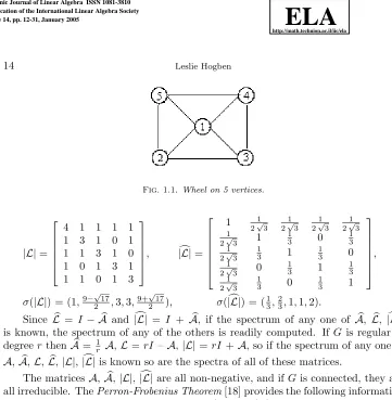
• Wn+1 is a wheel onn+1 vertices, i.e., a graph obtained by joining one addi-tional vertex to every vertex ofCn.
LetGbe a graph with vertices{1, . . . ,n}. We will discuss the following matrices associated withG.
• The adjacency matrix,A= [aij], whereaij = 1 if{i, j} is an edge ofGand
aij = 0 otherwise. Letσ(A) = (α1, . . . , αn).
• Thediagonal degree matrix,D= diag(degG1, . . . ,degGn).
• The√ normalized adjacency matrix,A=√D−1A√D−1, where D= diag(degG1, . . . ,
degGn). Let σ(A) = (ˆα1, . . . ,αˆn).
• TheLaplacian matrix,L=D − A. Letσ(L) = (λ1, . . . , λn).
• Thenormalized Laplacian matrix,L=√D−1 (D − A) √D−1 =I−A. Let σ(L) = (ˆλ1, . . . ,ˆλn).
• Thesignless Laplacian matrix,|L|=D+A. Letσ(|L|) = (µ1, . . . , µn).
• Thenormalized signless Laplacian matrix,
|L|=√D−1 (D+A)√D−1=I+A. Letσ(|L|) = (ˆµ1, . . . ,µˆn).
Example 1.1. For the wheel on five vertices, shown in Figure 1.1, the matrices
A,A,L,L,|L|, |L| and their spectra are
A=
0 1 1 1 1 1 0 1 0 1 1 1 0 1 0 1 0 1 0 1 1 1 0 1 0
, A=
0 1
2√3 1 2√3
1 2√3
1 2√3 1
2√3 0 1 3 0
1 3 1
2√3 1 3 0
1 3 0 1
2√3 0 1 3 0
1 3 1
2√3 1 3 0 1 3 0 ,
σ(A) = (−2,1−√5,0,0,1 +√5), σ(A) = (−2 3,−
1
3,0,0,1),
L=
4 −1 −1 −1 −1 −1 3 −1 0 −1 −1 −1 3 −1 0 −1 0 −1 3 −1 −1 −1 0 −1 3
, L=
1 2−√1 3
−1 2√3
−1 2√3
−1 2√3 −1
2√3 1 − 1
3 0 − 1 3 −1
2√3 − 1
3 1 − 1 3 0 −1
2√3 0 − 1
3 1 − 1 3 −1
2√3 − 1
3 0 − 1 3 1 ,
σ(L) = (0,3,3,5,5), σ(L) = (0,1,1,4 3,
Fig. 1.1.Wheel on 5 vertices. |L|=
4 1 1 1 1 1 3 1 0 1 1 1 3 1 0 1 0 1 3 1 1 1 0 1 3
, |L| =
1 1
2√3 1 2√3
1 2√3
1 2√3 1
2√3 1 1 3 0
1 3 1
2√3 1 3 1
1 3 0 1
2√3 0 1 3 1
1 3 1
2√3 1 3 0 1 3 1 ,
σ(|L|) = (1,9−√217,3,3,9+√217), σ(|L|) = (13,23,1,1,2).
Since L = I−A and |L| = I + A, if the spectrum of any one of A, L, |L|, is known, the spectrum of any of the others is readily computed. If Gis regular of degreerthenA= 1r A,L=rI –A,|L|=rI +A, so if the spectrum of any one of A,A,L, L,|L|,|L| is known so are the spectra of all of these matrices.
The matricesA,A,|L|,|L| are all non-negative, and ifGis connected, they are all irreducible. ThePerron-Frobenius Theorem[18] provides the following information about an irreducible non-negative matrixB (whereρ(B) denotes the spectral radius, i.e., maximum absolute value of an eigenvalue ofB).
1. ρ(B)>0.
2. ρ(B) is an eigenvalue ofB.
3. ρ(B) is algebraically simple as an eigenvalue ofB. 4. There is a positive vectorxsuch thatBx=ρ(B)x.
LetBbe a symmetric non-negative matrix. Eigenvectors for distinct eigenvalues ofB are orthogonal. IfBhas a positive eigenvectorxfor eigenvalueβ, then any eigenvector for a different eigenvalue cannot be positive, and soβ=ρ(B). Lete= [1,1, . . . ,1]T.
Then sinceA√De=√De,ρ(A) = 1, andρ(|L|) = 2.
The matricesA,D,A,L,L,|L|,|L| are also connected via the incidence matrix. The(vertex-edge) incidence matrixN of graphGwithnvertices andmedges is the n×m 0,1-matrix with rows indexed by the vertices of Gand columns indexed by the edges of G, such that the v, e entry of N is 1 (respectively, 0) if edge e is (respectively, is not) incident with vertexv. Then
N NT =
D+A=|L|and|L| = (√D−1 N) (√D−1N)T.
v,(w, v)-entry ofN′ is 1, thev,(v, w)-entry ofN′ is -1, and all other entries are 0. If G′ is any orientation ofGandN′ is the oriented incidence matrix then
N′N′T
=D − A=LandL= (√D−1N′) (√D−1N′)T.
SoL,|L|,L,|L|are all positive semidefinite, and so have non-negative eigenvalues. Theinertia of a matrix B is the ordered triple (i+, i−, i0), where i+ is the number of positive eigenvalues ofB,i− is the number of negative eigenvalues ofB, andi0 is the number of zero eigenvalues ofB. By Sylvester’s Law of Inertia [18], the inertia ofL is equal to the inertia ofL. Since L+|L| = 2I, the following facts have been established, providedGis connected.
1. σ(|L|)⊂[0,2] and ˆµn = 2 with eigenvector
√ De. 2. σ(A)⊂[−1,1] and ˆαn = 1 with eigenvector
√ De. 3. σ(L)⊂[0,2] and ˆλ1 = 0 with eigenvector√De. 4. λ1 = 0.
IfG is not connected, the multiplicity of 0 as an eigenvalue ofL is the number of connected components of G. For each of the matrices A, A, |L|, |L|, L, L the spectrum is the union of the spectra of the components.
IfAis the adjacency matrix of the line graphL(G) ofG(cf. [15]), then NT
N = 2I+A. It follows from theSingular Value Decomposition Theorem[18] that the non-zero eigenvalues ofN NT and
NT
N are the same (including multiplicities). Thus the spectrum of |L| is readily determined from that of the adjacency matrix of L(G). Since NT
N is positive semidefinite, the least eigenvalue of the adjacency matrix of L(G) is greater than or equal to -2. See [15] for further discussion of line graphs and graphs with adjacency matrix having all eigenvalues greater than or equal to -2.
We now turn our attention to information about the graph that can be extracted from the spectra of these matrices. This is the approach typically taken in Spectral Graph Theory.
The following parameters of graph G are determined by the spectrum of the adjacency matrix or, equivalently, by its characteristic polynomial
p(x) =xn+a
n−2xn−2+. . .+a1x+a0 (notean−1= 0 since tr A= 0). 1. the number of edges ofG= -an−2 = trA
2
2 =
α2i
2 2. the number of triangles ofG= -an−3
2 = trA
3
6 =
α3
i
6 .
The first equality in each of these statements is obtained by viewing the coefficient of p(x) as the sum of the principal minors of order k, the second is obtained by considering walks, and the third is obtained by using the fact that a real symmetric matrix is unitarily similar to a diagonal matrix.
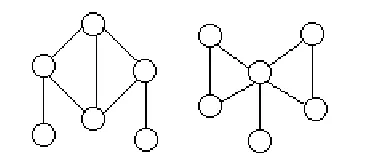
Unfortunately these results do not extend cleanly to longer cycles, as can be seen by considering the 4-cycle.
Fig. 1.2.Cospectral graphs withp(x) =−1 + 4x+ 7x2− 4x3−
7x4 +x6
.
A graphGis calledspectrally determinedif any graph with the same spectrum is isomorphic toG. Of course, one must identify the matrix (e.g., adjacency, Laplacian, etc.) from which the spectrum is taken. Examples of graphs that are spectrally determined by the adjacency matrix [11]:
• Complete graphs. • Empty graphs. • Graphs with one edge. • Graphs missing only 1 edge. • Regular graphs of degree 2.
• Regular graphs of degreen−3, wherenis the order of the graph.
However, “most” trees are not spectrally determined, in the sense that asngoes to infinity, the proportion of trees onnvertices that are determined by the spectrum of the adjacency matrix goes to 0 [28]; see also [11]. A recent survey of results on cospectral graphs and spectrally determined graphs can be found in [12].
There are many other graph parameters for which information can be extracted from the spectra of the various matrices associated with a graph. Here we mention only two examples, the vertex connectivity and the diameter.
A vertex cutset of G is a subset of vertices of G whose deletion increases the number of connected components of G. The vertex connectivity of G, κ0, is the minimum number of vertices in a vertex cutset (for a graph that is not the complete graph). The second smallest eigenvalue of the LaplacianL,λ2, is called the algebraic connectivity ofG.
Theorem 1.2. [14]; see also [15]If G is notKn, the vertex connectivity is greater than or equal to the algebraic connectivity, i.e.,λ2≤κ0.
The distance between two vertices in a graph is the length of (i.e., number of edges in) the shortest path between them. The diameter of a graph G, diam(G), is maximum distance between any two vertices of G.
Theorem 1.3. [5]The diameter of a connected graphGis less than the number of distinct eigenvalues of the adjacency matrix of G.
2. The Inverse Eigenvalue Problem of a Graph. Spectral Graph Theory originally focused on specific matrices, such as the adjacency matrix or the Lapla-cian matrix, whose entries are determined by the graph, with the goal of obtaining information about the graph from the matrices. In contrast, the Inverse Eigenvalue Problem of a Graph seeks to determine information about the possible spectra of the real symmetric matrices whose pattern of nonzero entries is described by a given graph.
We need some additional definitions and notation. For a symmetric realn×n matrix B, the graph of B, G(B), is the graph with vertices {1, . . . , n} and edges {{i, j}|bij = 0 andi =j}. Note that the diagonal ofB is ignored in determining
G(B).
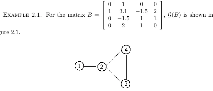
Example 2.1. For the matrix B =
0 1 0 0
1 3.1 −1.5 2 0 −1.5 1 1
0 2 1 0
[image:6.595.121.476.286.439.2], G(B) is shown in
Figure 2.1.
Fig. 2.1.The graph G(B)forBinExample 2.1.
LetSn be the set of real symmetricn×nmatrices. ForGa graph with vertices
{1, . . . , n}, define S(G) = {B ∈ Sn| G(B) = G}. Note that A, A, |L|, |L|, L,
L ∈ S(G). The Inverse Eigenvalue Problem of a Graph is to characterize the possible spectra of matrices inS(G).
The multiplicity of β as an eigenvalue of B ∈ Sn is denoted by mB(β). The
eigenvalueβ issimple ifmB(β) = 1. Themaximum multiplicity ofGis
M(G) = max{mB(β)|β∈σ(B), B∈ S(G)}, and theminimum rankofGis
mr(G) = min{rankB| B∈ S(G)}. SincemB(0) = dim kerB, it is clear that
M(G) + mr(G) = n. IfH is an induced subgraph ofGthen mr(H)≤mr(G). If G is not connected, then any matrix B ∈ S(G) is block diagonal, with the diagonal blocks corresponding to the connected components of G, and the spectrum ofB is the union of the spectra of the diagonal blocks. Thus we usually restrict our attention to connected graphs.
Characterizations of graphs of ordernhaving minimum rank 1, 2, andn– 1 have been obtained. For any graphG, a matrixB∈ S(G) with rankB≤n– 1 can always be obtained by takingC∈ S(G),γ∈σ(C), andB=C−γI. Thus, for any graphG, mr(G)≤n– 1. IfB∈ S(Pn), by deleting the first row and last column, we obtain an
Thus mr(Pn) =n– 1.
Theorem 2.2. [13] If for all B ∈ S(G), all eigenvalues of B are simple, then
G=Pn. Equivalently, mr(G) = n−1implies G=Pn.
For any graphGthat has an edge, any matrix inS(G) has at least two nonzero entries, so mr(G) ≥1. By examining the rank 1 matrix J (all of whose entries are 1), we see that mr(Kn) = 1. IfGis connected, then for any matrixB ∈ S(G), there
is no row consisting entirely of zeros. Any rank 1 matrixB with no row of zeros has all entries nonzero, and thus G(B) =Kn. Thus, for G a connected graph of order
[image:7.595.185.403.279.356.2]greater than one, mr(G) = 1 is equivalent toG=Kn.
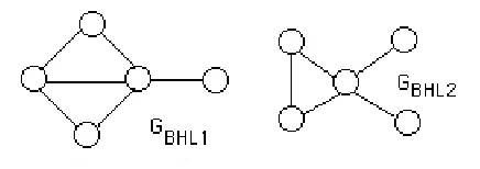
Fig. 2.2.Forbidden induced subgraphs formr(G) = 2.
Theorem 2.3. [4] A connected graph G has mr(G) ≤ 2 if and only if G does not contain as an induced subgraph any of: P4,K3,3,3(the complete tripartite graph), GBHL1 orGBHL2 (shown in Figure 2.2).
Additional characterizations of graphs having minimum rank 2 can be found in [4].
Recall that for any graphG, the diameter ofGis less than the number of distinct eigenvalues of the adjacency matrix of G(cf. Theorem 1.3), and the proof extends to show diam(G) is less than the number of distinct eigenvalues of any non-negative matrixB∈ S(G). IfT is a tree andB∈ S(T), it is possible to find a real numberγ and a 1,-1-diagonal matrixS such that ST S−1+γI is non-negative. Thus, we have the following theorem.
Theorem 2.4. [25] If T is a tree, for anyB ∈ S(T), the diameter of T is less than the number of distinct eigenvalues ofB.
There are many examples of treesT for which the minimum number of distinct eigenvalues is diam(T) + 1. Barioli and Fallat [1] gave an example of a tree for which the minimum number of distinct eigenvalues is strictly greater than this bound. Since n−(M(G)−1)≥the minimum number of distinct eigenvalues, for a treeT, diam(T)≤mr(T).
Most of the progress for trees is based on the Parter-Wiener Theorem and the interlacing of eigenvalues. IfB is ann×nmatrix,B(k) is the (n−1)×(n−1) matrix obtained fromB by deleting row and columnk. IfB∈ S(G), thenB(k)∈ S(G−k). LetB∈Sn andk∈ {1, . . . , n}. If the eigenvalues ofB areβ1≤β2. . .≤βn and the
eigenvalues ofB(k) areθ1 ≤θ2 ≤. . . ≤θn−1, then by the Interlacing Theorem [18]
β1≤θ1≤β2≤θ2. . .≤βn−1≤θn−1≤βn.
We sayk is a Parter-Wiener (PW) vertex of B for eigenvalueβ if mB(k)(β) =
mB(β) + 1;kis astrong PW vertexofBforβifkis a PW vertex ofB forβ andβis
an eigenvalue of at least three components ofG(B)−k. The next theorem is referred to as theParter-Wiener Theorem.
Theorem 2.6. [27], [29], [22] If T is a tree, B ∈ S(T) and mB(β) ≥ 2, then there is a strong PW vertex ofB forβ.
Corollary 2.7. IfT is a tree,B∈ S(T)andσ(B) = (β1, . . . , βn), thenβ1 and
βn are simple eigenvalues.
The set of high degree vertices of Gis H(G) = {k ∈ V(G)| degGk ≥3}. Only
high degree vertices can be strong PW vertices.
Example 2.8. The star onn+1 vertices,K1,n, has only one high degree vertex,
say vertex 1. Thus this vertex must be the strong PW vertex for any multiple eigen-value ofBwithG(B) =K1,n. By choosing the diagonal elements ofBfor 2, . . . , n+ 1
to be 0, we obtainmB(1)(0) =n and somB(0) =n−1 and mr(K1,n) = 2. (In this
case the other two eigenvalues are necessarily simple.)
As many people have observed, the Parter-Wiener Theorem need not be true for graphs that are not trees.
Example 2.9. For A the adjacency matrix of C4, m
A(0) = 2 but there is no PW vertex sinceC4−kisP3for any vertexk.
We define two more parameters of a graph that are related to maximum mul-tiplicity and minimum rank. The path cover number of G, P(G), is the minimum number of vertex disjoint paths occurring as induced subgraphs of Gthat cover all the vertices ofG, and ∆(G) = max{p−q|there is a set ofqvertices whose deletion leavesppaths}. These parameters are equal for trees, but not for all graphs.
Theorem 2.10. [19] For any treeT,M(T) =P(T) = ∆(T). For any graphG,
∆(G)≤M(G).
Theorem 2.11. [2] For any graphG,∆(G)≤P(G).
The relationship betweenM(G) andP(G) is less clear.
Example 2.12. The wheel on 5 vertices,W5, shown in Figure 1.1, has
P(W5) = 2 by inspection, and mr(W5) = 2 (by Theorem 2.3), so M(W5) = 3> P(W5).
Example 2.13. In [2], it is established that the penta-sun, H5, shown in
Fig-ure 2.3, has P(H5) = 3 > M(H5) = 2. More information on graphs for which P(G)> M(G) can be found in [2] and [3].
We now consider what combinations of eigenvalues and multiplicities are possible for trees. Since the first and last eigenvalue of a matrix whose graph is a tree must be simple, clearly the order is important in determining which lists of eigenvalues and multiplicities are possible. If the distinct eigenvalues of B are ˘β1 < . . . < β˘r with
multiplicitiesm1, . . . , mr, respectively, then (m1, . . . , mr) is called the ordered
multi-plicity list ofB. There has been extensive study of the possible ordered multiplicity lists of trees.
Theorem 2.14. [13], [20], [21]The possible ordered multiplicity lists of the follow-ing families of trees have been determined. Furthermore, if there is a matrixB∈ S(G)
Fig. 2.3.The penta-sunH5.
real numbers γ1< . . . < γr, there is a matrix in S(G) having eigenvalues γ1, . . . , γr with multiplicities m1, . . . , mr.
• Paths.
• Double Paths.
• Stars
• Generalized Stars
• Double Generalized Stars.
Thus for any of these graphs, determination of the possible ordered multiplicity lists of the graph is equivalent to the solution of the Inverse Eigenvalue Problem of the graph.
However, Barioli and Fallat [1] established that sometimes there are restrictions on which real numbers can appear as the eigenvalues for an attainable ordered mul-tiplicity list.
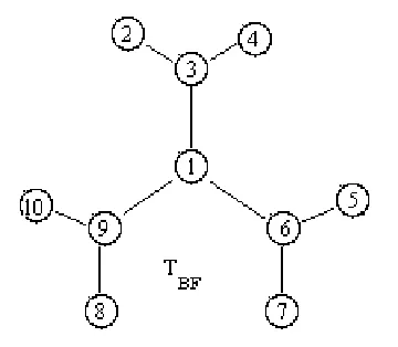
Fig. 2.4.A tree for which an ordered multiplicity list is possible only for certain real numbers.
[image:9.595.202.382.489.646.2]adjacency matrix isσ(A) = (−√5,−√2,−√2,0,0,0,0,√2,√2,√5), so the ordered multiplicity list ofAis (1,2,4,2,1). But the trace technique in [1] shows that ifB ∈ S(TBF) has the five distinct eigenvalues ˘β1 <β2˘ <β3˘ <β4˘ <β5˘ with multiplicities
mB( ˘β1) =mB( ˘β5) = 1, mB( ˘β2) =mB( ˘β4) = 2, mB( ˘β3) = 4, then ˘β1+ ˘β5= ˘β2+ ˘β4.
3. Generalized Laplacians and the Colin de Verdi`ere Number µ(G).
The symmetric matrix L= [lij] is a generalized Laplacian matrix ofGif for all i, j
withi=j,lij <0 ifiandj are adjacent inGandlij = 0 ifiandj are nonadjacent.
ClearlyLandLare generalized Laplacians. Note that ifLis a generalized Laplacian then −L has non-negative off-diagonal elements, and so there is a real number c such thatcI−L is non-negative. Thus, if Gis connected, by the Perron-Frobenius Theorem, the least eigenvalue of L is simple. Much recent work in Spectral Graph Theory with generalized Laplacians is based on Colin de Verdi`ere matrices and the Colin de Verdi`ere number µ(G). This graph parameter was introduced by Colin de Verdi`ere in 1990 ([7] in English). A thorough introduction to this important subject is provided by [17]. Here we list only a few of the definitions and results, following the treatment in [17].
The matrixLis a Colin de Verdi`ere matrix for graphGif 1. Lis a generalized Laplacian matrix ofG.
2. Lhas exactly one negative eigenvalue (of multiplicity 1).
3. (Strong Arnold Property) IfX is a symmetric matrix such thatLX= 0 and xi,j = 0 impliesi=j andi, jis not an edge of G, thenX = 0.
The Colin de Verdi`ere numberµ(G) is the maximum multiplicity of 0 as an eigenvalue of a Colin de Verdi`ere matrix. A Colin de Verdi`ere matrix realizing this maximum is called optimal. Note that condition (2) ensures that µ(G) is the multiplicity of λ2(L) for an optimal Colin de Verdi`ere matrix. The Strong Arnold Property is the requirement that certain manifolds intersect transversally. See [17] for more details.
Clearlyµ(G)≤M(G), since any Colin de Verdi`ere matrix is inS(G). There are many examples, such as Example 3.1 below, of matrices inS(G) where this inequality is strict, due to the failure of the Strong Arnold Property for matrices realizingM(G).
Example 3.1. The star K1,n has M(K1,n) = n−1 and this multiplicity is
attained (for eigenvalue 0) by the adjacency matrix. For n >3 (if the high degree vertex is 1), the matrixX = (e2−e3)(e4−e5)T + (e4
−e5)(e2−e3)T shows that
A does not have the Strong Arnold Property. In fact, µ(K1,n) = 2 (provided n > 2)
[17].
Acontractionof the graph Gis obtained by identifying two adjacent vertices of G, suppressing any loops or multiple edges that arise in this process. A minor of G arises by performing a series of deletions of edges, deletions of isolated vertices, and/or contraction of edges. Colin de Verdi`ere showed thatµis minor-monotone.
Theorem 3.2. [7]; see also [17]. If H is a minor ofGthenµ(H)≤µ(G).
The Strong Arnold Property is essential to this minor-monotonicity, as the fol-lowing example shows.
Example 3.3. Consider the graphGBHL2 shown in Figure 2.2. From [4],
mr(GBHL2) = 3, soM(GBHL2) = 2, but deletion of the edge that joins the two degree
The Robertson-Seymour theory of graph minors asserts that the family of graphs Gwithµ(G)≤k can be characterized by a finite set of forbidden minors [17]. Colin de Verdi`ere; Robertson, Seymour and Thomas; and Lov´asz and Schrijver have used this to establish the following characterizations.
Theorem 3.4. [7], [17]
1. µ(G)≤1 if and only if Gis a disjoint union of paths. 2. µ(G)≤2 if and only if Gis outerplanar.
3. µ(G)≤3 if and only if Gis planar.
4. µ(G)≤4 if and only if Gis linklessly embeddable.
A graph is planar if it can be drawn in the plane without crossing edges. A graph is outerplanar if it has such a drawing with a face that contains all vertices. An embedding of a graphGintoR3 islinklessif no disjoint cycles inGare linked in
R3. A graph is linklessly embeddableif it has a linkless embedding. See [17] for more detail.
Theorem 3.5. [15] LetL be a generalized Laplacian matrix of the graph Gwith
σ(L) = (ω1, ω2, . . . , ωn). IfG is2-connected and outerplanar then mL(ω2)≤2. IfG is3-connected and planar then mL(ω2)≤3.
4. Connections and New Results. Clearly there are close connections be-tween the recent work in Spectral Graph Theory on generalized Laplacians, and the Inverse Eigenvalue Problem of a Graph. Matrices attaining M(G) for eigenvalue 0 are central to this connection. Equivalently, we are concerned with matrices attaining the minimum rank of G. In particular, generalized Laplacian matrices realizing the minimum rank ofGare of interest.
We now turn to the question of whether we can realize the minimum rank ofG by a matrix inS(G) having some special form such as:
• the adjacency matrixA, • a 0,1- matrix,
• A+D forD a diagonal matrix, • a generalized Laplacian ofG.
Observation 4.1. For any graphG:
• The adjacency matrixAis a 0,1-matrix.
• Any0,1-matrixA∈ S(G)is of the formA+D for D a diagonal matrix.
• ForD a diagonal matrix,−(A+D)is a generalized Laplacian ofG.
• Finding a matrix of minimum rank inS(G)with off-diagonal elements non-negative is equivalent to finding a generalized Laplacian of minimum rank.
There are very few graphs for whichArealizes minimum rank. The starK1,n is
one such graph, but for the pathPn,Ais nonsingular ifnis even. We show that for
a tree, there is always a 0,1-matrix realizing minimum rank (equivalently, realizing maximal multiplicity for eigenvalue 0). This answers a question raised by Zhongshan Li [26].
Theorem 4.2. If T is a tree and Ais its adjacency matrix, then there exists a
vertices so that the result is isolated vertices (and one path with 2 vertices if the path had an even number of vertices originally). LetQ∗be the set ofq∗vertices consisting of the originalq vertices and the additional alternate interior vertices deleted. Then Q∗ has the property that T −Q∗ consists of p∗ disjoint paths, each having 1 or 2 vertices, and p∗−q∗ = M(T). Choose the diagonal elements of D corresponding to isolated vertices or to deleted vertices to be 0, and choose the diagonal elements of D corresponding to 2-vertex paths to be 1. Then 0 is an eigenvalue of each of the p∗ paths and, by interlacing, m
A+D(0) ≥ p∗−q∗ = M(T)≥ mA+D(0). Thus
rank(A+D) =n−mA+D(0) =n−M(T) = mr(T).
By using the algorithm of Johnson and Saiago [24] to produce the initial setQof vertices to delete, we obtain the following algorithm for producing a 0,1-matrixA+D of minimum rank among matrices inS(T). As in [24], δT(v) = degTv−degH(T)v, whereH(T) is the subgraph of T induced by the vertices of degree at least 3 inT.
Algorithm 4.3.
1. Set T′=T and Q=∅. Repeat:
a) Q′ ={v | δT′(v)≥2}, b) Set T′=T′−Q′. c) Set Q=Q∪Q′. Until Q′=∅. This determines Q.
2. In each path, remove alternate interior vertices and add these vertices to Q to obtain Q∗.
3. Choose D = diag(d1, . . . , dn) where dk = 1 if k /∈Q∗ and the path of
[image:12.595.145.435.460.603.2]T−Q∗ containing k has 2 vertices; otherwise, dk = 0.
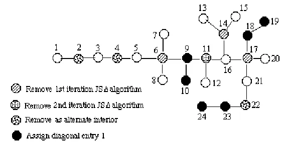
Fig. 4.1.ApplyingAlgorithm 4.3to a tree T.
Example 4.4. Figure 4.1 illustrates the application of Algorithm 4.3 to the tree
vertices in Figure 4.1, are assigned 1, and all other diagonal entries (including those corresponding to both shaded and unshaded vertices) are assigned 0. Thus with
D= diag(0,0,0,0,0,0,0,0,1,1,0,0,0,0,0,0,0,1,1,0,0,0,1,1), A+D is a 0,1-matrix inS(T) with rank(A+D) = 17 = mr(T).
Algorithm 4.3 will produce the adjacency matrix ofT ifAattains the minimum rank of T. Theorem 4.2 need not be true for graphs that are not trees, that is, we cannot always find a 0,1-matrix inS(G) realizing minimum rank. In particular, it is impossible for the 5-cycle.
Theorem 4.5. For any n-cycle Cn, n ≥ 3, rank(A −2 cos(2π
n)I) = n−2 =
mr(Cn). Furthermore, there is a 0,1-matrixD with rank(A+D) = mr(Cn) if and only ifn= 5. Specifically, the diagonal matrices D listed below have this property.
0. If n ≡ 0 mod 4 then let D = diag(0,0, . . . ,0), i.e., the adjacency matrix realizes minimum rank.
1. If n≡1mod4 andn≥9 then letD= diag(1,1,1,1,1,1,1,1,1,0,0, . . .,0).
2. If n≡2mod4 then let D= diag(1,1,1,1,1,1,0,0, . . . ,0).
3. If n≡3mod4 then let D= diag(1,1,1,0, . . . ,0). If n≡0mod3 thenD=I also works.
Proof. It is known [10] that the eigenvalues ofAare 2 cos(2πkn ) fork= 1, . . . , n.
Since cos(2π
n) = cos(
2π(n−1)
n ), it is clear that rank(A −2 cos(
2π
n)I) =n−2≥mr(Cn).
Since Pn−1 is an induced subgraph of Cn, mr(Cn) ≥ n−2, establishing the first
statement.
Direct examination of all 32 possibilities for the diagonal shows that all 0,1-matrices inS(C5) are nonsingular and thus do not realize mr(C5) = 3.
For each general case, we exhibit two vectorsz1 andz2 in the kernel of A+D. Each vector has a repeatable block of 4 entries (or 3 entries forn≡0 mod 3) that is used as many times as necessary to obtain a vector of the right length. Such a block will be denoted repeat[. . . ].
Determination ofD based on congruence mod 4: 0. Letn≡0 mod 4 andD= diag(0,0, . . . ,0).
Thenz1= (repeat[−1,0,1,0])T andz2= (repeat[0,
−1,0,1])T.
1. Letn≡1 mod 4 andD= diag(1,1,1,1,1,1,1,1,1,0,0, . . .,0). Thenz1= (−1,1,0,−1,1,0,−1,1,0, repeat[−1,0,1,0])T and
z2= (0,−1,1,0,−1,1,0,−1,1, repeat[0,−1,0,1])T.
2. Letn≡2 mod 4 andD= diag(1,1,1,1,1,1,0,0, . . . ,0). Thenz1= (−1,1,0,−1,1,0, repeat[−1,0,1,0])T and
z2= (0,−1,1,0,−1,1, repeat[0,−1,0,1])T.
3. Letn≡3 mod 4 andD= diag(1,1,1,0, . . . ,0). Thenz1= (−1,1,0, repeat[−1,0,1,0])T and
z2= (0,−1,1, repeat[0,−1,0,1])T.
Forn≡0 mod 3,D=I, letz1= (repeat[−1,1,0])T andz2= (repeat[0,
−1,1])T. Corollary 4.6. For every wheel Wn+1, n ≥ 4, there is a diagonal matrix D such that rank(A+D)= mr(Wn+1).
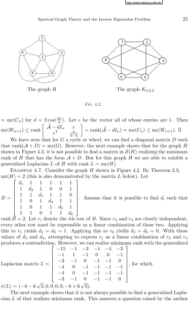
The graphH The graphK2,2,2
Fig. 4.2.
= mr(Cn) for d = 2 cos(2nπ). Let e be the vector all of whose entries are 1. Then
mr(Wn+1)≤rank
A −dIn e
eT n
2−d
= rank(A − dIn) = mr(Cn)≤mr(Wn+1).
We have seen that forGa cycle or wheel, we can find a diagonal matrixD such that rank(A+D) = mr(G). However, the next example shows that for the graphH shown in Figure 4.2, it is not possible to find a matrix inS(H) realizing the minimum rank ofH that has the formA+D. But for this graphH we are able to exhibit a generalized LaplacianL ofH with rankL= mr(H).
Example 4.7. Consider the graphH shown in Figure 4.2. By Theorem 2.3,
mr(H) = 2 (this is also demonstrated by the matrixLbelow). Let
B =
d1 1 1 1 1 1 1 d2 1 0 0 1 1 1 d3 1 1 0 1 0 1 d4 1 1 1 0 1 1 d5 1
1 1 0 1 1 d6
. Assume that it is possible to find di such that
rankB= 2. Letri denote theith row ofB. Sincer3 andr4 are clearly independent,
every other row must be expressible as a linear combination of these two. Applying this to r5 yields d4 = d5 = 1. Applying this to r6 yields d3 =d6 = 0. With these values of d3 and d4, attempting to expressr1 as a linear combination ofr3 and r4 produces a contradiction. However, we can realize minimum rank with the generalized
Laplacian matrixL=
−15 −1 −3 −4 −4 −3 −1 1 −1 0 0 −1 −3 −1 0 −1 −1 0 −4 0 −1 −1 −1 −1 −4 0 −1 −1 −1 −1 −3 −1 0 −1 −1 0
, for which
σ(L) = (−8−6√3,0,0,0,0,−8 + 6√3).
[16].
Example 4.8. Consider the graphK2,2,2 shown in Figure 4.2.
The matrixB =
0 1 1 0 1 1
1 −3 −2 1 0 −1 1 −2 −1 1 1 0
0 1 1 0 1 1
1 0 1 1 3 2
1 −1 0 1 2 1
∈ S(K2,2,2) has rankB = 2.
Now let matrixM ∈ S(K2,2,2). Det[1,2,3; 4,5,6] =m15m26m34+m16m24m35,
so if M is non-negative, Det[1,2,3; 4,5,6]>0 and rankM ≥3. Thus the minimum rank of K2,2,2 can not be realized by a matrix in S(K2,2,2) with non-negative
off-diagonal entries. Equivalently, the minimum rank ofK2,2,2 can not be realized by a generalized Laplacian.
Even though it is not always possible to find a matrix realizing minimum rank that has one of the special forms adjacency matrix (i.e., 0,1-matrix with all diagonal entries 0), 0,1-matrix, adjacency matrix + diagonal matrix, generalized Laplacian matrix, there are many graphs for which it is possible. The next two theorems offer ways to obtain matrices of special form realizing minimum rank for graphs that have acut-vertex, that is the vertex in a singleton cutset. As in [2], therank spreadofvin G,rv(G) = mr(G) – mr(G−v). Letv be a cut-vertex of Gand letGi, i= 1, . . . , h
be the components of G−v. Let Gi be the subgraph of G induced by v and the
vertices of Gi. G is called thevertex-sum of G1, . . . , Gh and it is shown in [2] that
rv(G) = minhi=1rv(Gi), 2
.
Theorem 4.9. Suppose the graphGis the vertex-sum atv of the graphs Gi, for
i= 1, . . . , h, and rv(G) = 2. LetGi=Gi−v. If there exist matricesA1, . . . , Ah such that fori= 1, . . . , h,
• Ai∈ S(Gi),
• rankAi= mr(Gi),
• Ai is of typeX,
then there exists a matrixA with
• A∈ S(G),
• rankA= mr(G),
• Ais of typeX
for X any of the following types of matrix: adjacency matrix, 0,1-matrix, sum of a diagonal matrix and the adjacency matrix, generalized Laplacian matrix.
Proof. Without loss of generality, assume v = 1, the vertices of G1 are next, followed by the vertices ofG2, etc. Since r1(G) = 2, mr(G) = mr(G−1) + 2 =
mr(Gi) + 2. LetA=A1 ⊕. . .⊕Ah. ClearlyA∈ S(G−1), rankA= mr(G−1),
and if Ai is of type X for all i, then so is A. Define A=
0 bT
b A
wherebi =t if
{i,1}is an edge ofGandbi= 0 otherwise. Chooset= 1 ifX is the class of adjacency
mr(G).
[image:16.595.209.377.188.292.2]We illustrate this theorem in the next two examples.
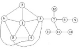
Fig. 4.3. A graph to whichTheorem 4.9can be applied to produce a generalized Laplacian of minimum rank.
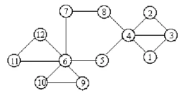
Example 4.10. For the graph Gshown in Figure 4.3, vertex 7 is a cut-vertex.
The components ofG−7 are the induced subgraphs1,2,3,4,5,6,8,9,10, and 11,12,13, having minimum ranks 2,1,0, and 2, respectively. Since mr(7,10) = 1 and mr(10) = 0, r7(7,10) = 1. Similarly, r7(7,8,9) = 1. Since rv(G) =
minhi=1rv(Gi), 2
, r7(G) = 2. Thus mr(G) = (2 + 1 + 0 + 2) + 2 = 7. We can apply Theorem 4.9, Example 4.7, and Algorithm 4.3 to produce a generalized LaplacianLhaving rankL= 7. The matrix produced is
L=
−15 −1 −3 −4 −4 −3 0 0 0 0 0 0 0
−1 1 −1 0 0 −1 0 0 0 0 0 0 0
−3 −1 0 −1 −1 0 −1 0 0 0 0 0 0 −4 0 −1 −1 −1 −1 0 0 0 0 0 0 0 −4 0 −1 −1 −1 −1 0 0 0 0 0 0 0
−3 −1 0 −1 −1 0 0 0 0 0 0 0 0
0 0 −1 0 0 0 0 −1 0 −1 0 −1 0
0 0 0 0 0 0 −1 −1 −1 0 0 0 0
0 0 0 0 0 0 0 −1 −1 0 0 0 0
0 0 0 0 0 0 −1 0 0 0 0 0 0
0 0 0 0 0 0 0 0 0 0 0 −1 0
0 0 0 0 0 0 −1 0 0 0 −1 0 −1
0 0 0 0 0 0 0 0 0 0 0 −1 0
.
Example 4.11. For the graphG shown in Figure 4.4, vertex 8 is a cut-vertex
of G. We showr8(G) = 2: Let G1 = 8,10,11,12,13,14,15; mr(G1) = 5 because G1=P7 andP6 is an induced subgraph ofG1. The minimum rank of the six cycle 10,11,12,13,14,15is 4, sor8(G1) = 1. Sincer8(8,9) = 1,r8(G) = 2.
Fig. 4.4.A graph to whichTheorem 4.9can be applied to produce a0,1-matrix of minimum rank.
When we apply Theorem 4.9 to the sum at vertex 8, the diagonal matrix produced isD = diag(0,1,1,1,0,1,1,0,0,1,1,1,1,1,1).
We can check that for this D, A+D is a minimum rank matrix by verifying rank(A+D) = 10 and showing this is the minimum rank ofG. Since the components ofG2−1 are2,3,4,5, and6,7, having minimum ranks 1,0,and 1,respectively, andr1(G2) = 2, mr(G2) = 4. Since the components ofG−8 areG2,9, and the six cycle, having minimum ranks 4,0, and 4,respectively, andr8(G) = 2, mr(G) = 10.
Theorem 4.12. Suppose the graph G is the vertex-sum at v of the graphs Gi, for i = 1, . . . , h and rv(G) = 0. If there exist matrices A1, . . . , Ah such that for
i= 1, . . . , h,
• Ai∈ S(Gi),
• rank Ai = mr(Gi),
• Ai is of typeX,
then there exists a matrixA with
• A∈ S(G),
• rank A = mr(G),
• Ais of typeX
for X one of the classes: adjacency matrix, sum of a diagonal matrix and the adja-cency matrix, generalized Laplacian matrix.
Proof. Since by [2],rv(G) = min{rv(Gi),2}, andrv(G) = 0, clearly
rv(Gi) = 0 fori= 1, . . . , h. Thus mr(Gi) = mr(Gi−v) fori= 1, . . . , h. Then
mr(G) = mr(G−v) + 0 =mr(Gi−v) = mr(Gi).
Fori= 1, . . . , h, let ˘Ai be then×nmatrix obtained fromAi by embedding it in
the appropriate place (setting all other entries 0). LetA= ˘A1+. . .+ ˘Ah. IfAi∈ X
for alli, then so isA(the only entry that is the sum of more than one nonzero entry is thev, v-entry). And rank A ≤rank Ai = mr(Gi) = mr(G) ≤rank A, so
rankA= mr(G).
We illustrate this theorem in the next example.
Example 4.13. The graphGshown in Figure 4.5 is the vertex-sum at 4 of the
Fig. 4.5.A graph to whichTheorem 4.12can be applied to produce a matrix of minimum rank that is the sum of the adjacency matrix and a diagonal matrix.
mr(G1−4).
The graph G1 is the vertex sum at 6 of 4,5,6,7,8, 6,9,10, and 6,11,12. Since mr(4,5,6,7,8) = mr(4,5,7,8) = 3, r6(4,5,6,7,8) = 0. Similarly,
mr(6,9,10) = 1,r6(6,9,10) = 0, mr(6,11,12) = 1, andr6(6,11,12) = 0. Thus, r6(G1) = 0 and mr(G1) = 5.
Likewise,G1−4 is the vertex sum at 6 of5,6,6,7,8,6,9,10, and6,11,12. Since mr(5,6) = 1 and mr(5) = 0, r6(5,6) = 1. Similarly, r6(6,7,8) = 1, so r6(G1−4) = 2. Thus, mr(G1−4) =mr(5)+ mr(7,8)+ mr(9,10)+ mr(11,12) + r6(G1−4) = 5. Since mr(G1) = mr(G1−4), r4(G1) = 0.
Thus, mr(G) =mr(G1−4)+ mr(1,2,3)+r4(G) = 7. We can apply Theorem 4.12 (twice) and Theorem 4.5 to produce a diagonal matrixD such that rankA+D = 7. The matrixA+D is built from
A1=
0 0 1 1 0 0 1 1 1 1 1 1 1 1 1 1
∈ S(1,2,3,4),
A2=
1−√5
2 1 0 0 1 1 1−2√5 1 0 0 0 1 1−2√5 1 0 0 0 1 1−√5
2 1 1 0 0 1 1−2√5
∈ S(4,5,6,7,8),
andA3=A4=
1 1 1 1 1 1 1 1 1
∈ S(6,9,10) =S(6,11,12).
Note A1 and A2 will overlap on vertex 4, andA2, A3 and A4 overlap on vertex 6. The diagonal matrix produced is
D= (0,0,1,1 +1−√5 2 ,
1−√5 2 ,2 +
1−√5 2 ,
1−√5 2 ,
1−√5
2 ,1,1,1,1).
REFERENCES
[1] F. Barioli and S. M. Fallat. On two conjectures regarding an inverse eigenvalue problem for acyclic symmetric matrices.Electronic Journal of Linear Algebra, 11:41–50, 2004. [2] F. Barioli, S. Fallat, and L. Hogben. Computation of minimal rank and path cover number for
graphs. Linear Algebra and its Applications, 392:289–303, 2004.
[3] F. Barioli, S. Fallat, and L. Hogben. On the difference between the maximum multiplicity and path cover number for tree-like graphs. To appear inLinear Algebra and its Applications. [4] W. W. Barrett, H. van der Holst, and R. Loewy. Graphs whose minimal rank is two.Electronic
Journal of Linear Algebra, 11:258-280, 2004.
[5] R. A. Brualdi and H. J. Ryser. Combinatorial Matrix Theory. Cambridge University Press, Cambridge, 1991.
[6] F. R. K. Chung. Spectral Graph Theory, CBMS 92, American Mathematical Society, Provi-dence, 1997.
[7] Y. Colin de Verdi`ere. On a new graph invariant and a criterion for planarity. InGraph Structure Theory, pp. 137–147. Contemporary Mathematics 147, American Mathematical Society, Providence, 1993.
[8] Y. Colin de Verdi`ere. Multiplicities of eigenvalues and tree-width graphs. Journal of Combi-natorial Theory, Series B, 74:121–146, 1998.
[9] D. M. Cvetcovi´c, M. Doob, I. Gutman, and A. TorgaˇsevRecent Results in the Theory of Graph Spectra. North-Holland, Amsterdam, 1988.
[10] D. M. Cvetcovi´c, M. Doob, and H. Sachs Spectra of Graphs. Academic Press, Inc., New York, 1980.
[11] D. Cvetcovi´c, P. Rowlinson, and S. Simi´c Eigenspaces of graphs. Cambridge University Press, Cambridge, 1997.
[12] E. R. van Dam and W. H. Haemers. Which graphs are determined by their spectrum? Linear Algebra and its Applications, 373:241–272, 2003.
[13] M. Fiedler. A characterization of tridiagonal matrices. Linear Algebra and its Applications, 2:191–197, 1969.
[14] M. Fiedler. Algebraic connectivity in graphs.Czechoslovak Mathematical Journal, 23:298–305, 1973.
[15] C. Godsil and G. Royle Algebraic Graph Theory. Springer-Verlag, New York, 2001.
[16] L. Hogben. Spectral graph theory and the inverse eigenvalue of a graph. Presentation at Di-rections in Combinatorial Matrix Theory Workshop, Banff International Research Station, May 7–8, 2004.
[17] H. van der Holst, L. Lov´asz, and A. Shrijver. The Colin de Verdi`ere graph parameter. In Graph Theory and Computational Biology (Balatonlelle, 1996), pp. 29–85. Mathematical Studies, Janos Bolyai Math. Soc., Budapest, 1999.
[18] R. Horn and C. R. Johnson. Matrix Analysis. Cambridge University Press, Cambridge, 1985. [19] C. R. Johnson and A. Leal Duarte. The maximum multiplicity of an eigenvalue in a matrix
whose graph is a tree. Linear and Multilinear Algebra, 46:139–144, 1999.
[20] C. R. Johnson and A. Leal Duarte. On the possible multiplicities of the eigenvalues of a Hermitian matrix the graph of whose entries is a tree.Linear Algebra and its Applications, 348:7–21, 2002.
[21] C. R. Johnson, A. Leal Duarte, and C. M. Saiago. Inverse Eigenvalue problems and lists of multiplicities for matrices whose graph is a tree: the case of generalized stars and double generalized stars. Linear Algebra and its Applications, 373:311–330, 2003.
[22] C. R. Johnson, A. Leal Duarte, and C. M. Saiago. The Parter-Wiener theorem: refinement and generalization. SIAM Journal on Matrix Analysis and Applications, 25:311–330, 2003. [23] C. R. Johnson, A. Leal Duarte, C. M. Saiago, B. D. Sutton, and A. J. Witt. On the relative
position of multiple eigenvalues in the spectrum of an Hermitian matrix with given graph. Linear Algebra and its Applications, 363:352–361, 2003.
[24] C. R. Johnson and C. M Saiago. Estimation of the maximum multiplicity of an eigenvalue in terms of the vertex degrees of the graph of the matrix. Electronic Journal of Linear Algebra, 9:27–31, 2002.
symmetric matrix whose graph is a given tree.Mathematical Inequalities and Applications, 5:175–180, 2002.
[26] Z. Li. On Minimum Ranks of Sign Pattern Matrices. Presentation atDirections in Combina-torial Matrix Theory Workshop, Banff International Research Station, May 7–8, 2004. [27] S. Parter. On the eigenvalues and eigenvectors of a class of matrices. Journal of the Society
for Industrial and Applied Mathematics, 8:376–388, 1960.
[28] A. J. Schwenk. Almost all trees are cospectral. In New Directions in the Theory of Graphs (Proc. Third Ann Arbor Conference at the University of Michigan), pp. 275–307. Academic Press, New York, 1973.