Strictly Convex Drawings of Planar Graphs
Imre B´ar´any and G¨unter Rote
Received: July 13, 2005 Revised: June 21, 2006
Communicated by G¨unter Ziegler
Abstract. Every three-connected planar graph withn vertices has a drawing on an O(n2)
×O(n2) grid in which all faces are strictly
convex polygons. These drawings are obtained by perturbing (not strictly) convex drawings onO(n)×O(n) grids. Tighter bounds are obtained when the faces have fewer sides. In the proof, we derive an explicit lower bound on the number of primitive vectors in a triangle.
2000 Mathematics Subject Classification: Primary 05C62; Secondary 52C05.
Keywords and Phrases: Graph drawing, planar graphs.
1 Introduction
A strictly convex drawing of a planar graph is a drawing with straight edges in which all faces, including the outer face, are strictly convex polygons, i. e., polygons whose interior angles are less than 180◦.
Theorem 1. (i) A three-connected planar graph with n vertices in which every face has at most k edges has a strictly convex drawing on an
O(nw)×O(n2k/w)grid of areaO(n3k), for any choice of a parameterw in the range1≤w≤k.
(ii) In particular, every three-connected planar graph with n vertices has a strictly convex drawing on anO(n2)
×O(n2)grid, and on anO(n)
×O(n3) grid.
When referring to aW×H grid of widthW and heightH, the constant hidden in theO-notation is on the order of 100 for the width and on the order of 10000 for the height. This is far too much for applications where one wants to draw graphs on a computer screen, for example. For the case w = 1, the bound is tighter: the grid size is approximately 14n×30n2k. For part (iii) of the
theorem, the grid size is at most 14n×14n, and if the outer face is a triangle, it is 2n×2n.
The main idea of the proof is to start with a (non-strictly) convex embedding, in which angles of 180◦are allowed, and to perturb the vertices to obtain strict convexity. We will use an embedding with special properties that is provided by the so-calledSchnyder embeddings, which are introduced in Section 2.
Historic context. The problem of drawing graphs with straight lines has a long history. It is related to realizing connected planar graphs as three-dimensional polyhedra. By a suitable projection on a plane, one obtains from a polyhedron a straight-line drawing, a so-calledSchlegel diagram. The faces in such a drawing are automatically strictly convex. By a projective transforma-tion, it can be arranged that the projection along a coordinate axis is possible, and hence a suitable realization as a grid polytope gives rise to a grid drawing of the graph. However, the problem of realizing a graph as a polytope is more restricted: not every drawing with strictly convex faces is the projection of a polytope. In fact, there is an exponential gap between the known grid size for strictly convex planar drawings and for polytopes in space.
The approaches for realizing a graph as a polytope or for drawing it in the plane come in several flavors. The classical methods of Steinitz (for polytopes) and F´ary and Wagner (for graphs) work incrementally, making local modifications to the graph and adapting the geometric structure accordingly. Tutte [15, 16] gave a “one-shot” approach for drawing graphs that sets up a system of equa-tions. This method yields also a polytope via the Maxwell-Cremona correspon-dence, see [11]. All these methods give embeddings that can be drawn on an integer grid but require an exponential grid size (or even larger, if one is not careful).
The first methods for straight-line drawings of graphs on anO(n)×O(n) grid were proposed for triangulated graphs, independently by de Fraysseix, Pach and Pollack [7] and by Schnyder [13]. The method of de Fraysseix, Pach and Pollack [7] is incremental: it inserts vertices in a special order, and modifies a partial grid drawing to accommodate new vertices. In contrast, Schnyder’s method is another “one-shot” method: it constructs some combinatorial struc-ture in the graph, from which the coordinates of the embedding can be readily determined afterwards. Both methods work in linear time. O(n)×O(n) is still the best known asymptotic bound on the size of planar grid drawings.
convex (but not necessarily strictly convex) drawings with O(n)×O(n) size, for example by Chrobak and Kant [5] (`a la Fraysseix, Pach and Pollack); or Schnyder and Trotter [14] and Felsner [8], see also [4] (`a la Schnyder). Our algorithm builds on the output of Felsner’s algorithm, which is described in the next section. Luckily, this embedding has some special features, which our algorithm uses.
The idea of getting a strictly convex drawing by perturbing a convex drawing was pioneered by Chrobak, Goodrich and Tamassia [6]. They claimed to con-struct strictly convex embeddings on an O(n3)×O(n3) grid, without giving full details, however. This was improved toO(n7/3)
×O(n7/3) in [12]. In this
paper we further improve the “fine perturbation” step of [12] to obtain a bound ofO(n2)
×O(n2) for grid drawings. Theorem 1 gives better bounds when the
faces have few sides, and we allow grids of different aspect ratios (keeping the same total area).
In the course of the proof, we need explicit (not just asymptotic) lower bounds on the number of primitive vectors in certain triangles. A primitive vector is an integer vector which is not a multiple of another integer vector; hence, primitive vectors can be used to characterize the directions of polygon edges. The existence of many short primitive vectors is the key to constructing strictly convex polygons with many sides. These lower bounds are derived in Section 5, based on elementary techniques from the geometry of numbers.
2 Preliminaries: Schnyder Embeddings of Three-Connected Plane Graphs
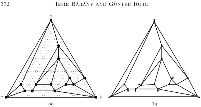
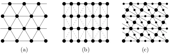
Felsner [8] (see also [9, 4]) has extended the straight-line drawing algorithm of Schnyder, which works for triangulated planar graphs, to arbitrary three-connected graphs. It constructs a drawing with special properties, beyond just having convex faces. These properties will be crucial for the perturbation step. Felsner’s algorithm works roughly as follows. The edges of the graph are covered by three directed trees which are rooted at three selected vertices a, b, c on the boundary, forming aSchnyder wood. The three trees define for each vertex v three paths from v to the respective root, which partition the graph into three regions. Counting the faces in each region gives three numbers x, y, z which can be used as barycentric coordinates for the point v with respect to the points a, b, and c. Selectingabc as an equilateral triangle of side length f−1 (the number of interior faces of the graph) yields vertices which lie on a hexagonal grid formed by equilateral triangles of side length 1, see Figure 1a. Sincef ≤2nthis yields a drawing on a grid of size 2n×2n.
This straight-line embedding has the following important property (see [8, Lemma 4 and Figure 11], [4, Fact 5]):
(a) (b)
a b
c
Figure 1: (a) A Schnyder embedding on a hexagonal grid and (b) on the refined grid after the initial (rough) perturbation
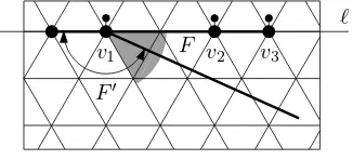
From this it follows immediately that there can be no angle larger than 180◦, and hence all faces are convex. Moreover, it follows that the interior faces F have theEnclosing Triangle Property, see Figure 4a ([8, proof of Lemma 7], [4, Lemma 2]):
The Enclosing Triangle Property. Consider the line x = const through the point ofF with maximumx-coordinate, and similarly for the other three coordinate directions. These three lines form a triangle TF which encloses F. Then all vertices of F lie on the
boundary ofTF, butF contains none of the vertices ofTF.
It follows that interior faces with k ≤ 4 sides are already strictly convex. Throughout, we will callTF theenclosing triangle of the faceF.
The Schnyder wood and the coordinates of the points can be calculated in linear time. Recently, Bonichon, Felsner, and Mosbah [4], have improved the grid size to (n−2)×(n−2). However, the resulting drawing does not have the Three Wedges Property. An alternative algorithm for producing an embedding with a property similarly to the Enclosing Triangle Property is sketched in Chrobak, Goodrich and Tamassia [6]. It proceeds incrementally in the spirit of the algorithm of de Fraysseix, Pach and Pollack [7] and takes linear time. From the details given in [6] it is not clear whether the embedding has also the Three Wedges Property, which we need for our algorithm. The original algorithm of Chrobak and Kant [5] achieves a weak form of the Three Wedges Property, where F is permitted to contain vertices ofTF. Maybe, this algorithm can be
v v
(a) (b)
150◦
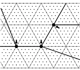
Figure 2: (a) Each closed shaded wedge contains exactly one edge incident to v. There may be additional edges in the interior of the white sectors. (b) A typical situation at a vertex which is perturbed.
Figure 3: The three possible new positions for a single vertex in the rough perturbation. (Only the three boundary verticesa,b,care pushed in directions opposite to these.)
3 Rough Perturbation
Before making all faces strictly convex, we perform an initial perturbation on a refined grid which is smaller by only a constant factor. This preparatory step will ensure that the subsequent “fine perturbation” can treat each face independently.
We overlay a triangular grid which is scaled by a factor of 1/7, see Figures 3 and 5. A point may be moved to one of the three possible positions shown in Figure 3, by a distance of √3/7. The precise rules are as follows: A vertex v on an interior faceF is moved if and only if the following two conditions hold.
(i) The interior angle ofF atv is larger than 150◦ (including the possibility of a straight angle of 180◦); and
(ii) vis incident to an edge ofF which lies on the enclosing triangleTF.
F TF
(a) (b) (c)
?
? ?
Figure 4: (a) A typical faceF constructed by the convex embedding algorithm. (b) The new positions of the vertices ofF which are pushed out are indicated. (c) The result of the rough perturbation. The perturbation of the vertices with question marks depends on the other faces incident to these vertices.
toF andvthecritical angle ofv. For a boundary vertex different froma, b, c, the exterior angle is the critical angle, but these vertices are not subject to the rough perturbation. The three corners a, b, andc are treated specially: they are pushed straight intothe triangle by the rough perturbation, as illustrated in Figure 1. Examples can be seen in Figure 4b–c and Figure 5. The result of
Figure 5: Example of the rough perturbation.
perturbing the example in Figure 1a is shown in Figure 1b.
There can be no conflict in applying the rules by regarding a vertex vas part of different faces: the bound of 150◦ on the angle, together with the Three Wedges Property ensures that there is at most one critical angle for every vertex (Figure 2b).
The result has the following properties:
Lemma 1. After the rough perturbation, all faces are still convex.
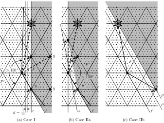
ℓ ℓ
r d= 1
14
ℓ s
ℓ′′
>150◦ x x x
F′
F F
y ≤150◦
y F
z z
z z
z
z
y
ℓ′
(a) Case I (b) Case IIa (c) Case IIb
y y
Figure 6: The cases in the proof of Lemma 1. The figures show possible locations for the neighborsy andzofx.
Proof. It is evident that no critical angle can become bigger than 180◦. For non-critical angles, this is also easy to see (cf. Figure 4c). (In fact, the second statement is a strengthening of this claim.)
We now prove this second statement of the lemma by considering different cases. The reader who is satisfied with the existence of some small enough perturbation boundε >0 may skip the rest of the proof. We continue to show that we can chooseε= 1/30.
Consider a non-critical angleyxzat a vertexxin a faceF. We assume without loss of generality thatxlies on thelower left edgeℓof the enclosing triangleTF.
Case I. The point xis incident to a critical angle of another faceF′, and thus xis pushed out ofF′.
Without loss of generality, we can assume thatx lies on the lower right edge of TF′, and thus xis perturbed in the lower right direction, as in Figure 6a.
(The other case, whenxlies on the upper edge ofTF′ and is pushed vertically
the enclosing triangle TF. Thus,y and z are restricted to the shaded area in
Figure 6a. Even if all three points are perturbed by the rough perturbation, they are still separated by a vertical strip of width d= 1
2 −2· 3 14 =
1 14. An
additional perturbation of 1 30 <
1
2·14 cannot make the angle at xlarger than
180◦.
Case II. The pointxnot perturbed by the initial perturbation. Case IIa. The pointxhas a neighbor onℓ.
We can assume w.l.o.g. that it is the lower neighbory, see Figure 6b. The angle yxzmust be at most 150◦because otherwisexwould be critical. It means that z cannot lie to the left ofx, and thusyandzare restricted to the shaded area in Figure 6b. Even if they are perturbed, they remain above the lines, which is obtained by offsetting the edge of the shaded region that is closest tox. The distance fromxtosis 1/7·p
3/7≈0.0935> 302. Thus, there is enough space to additionally perturb the pointsx,yandzwithout creating a concave angle. (Actually, the vertex xwill not even be perturbed in the fine perturbation.) Case IIb. The pointxhas no neighbors onℓ, see Figure 6c.
This means that y and z lie on or beyond the next grid line ℓ′ parallel to ℓ. The rough perturbation can move them closer to ℓ, but they remain beyond another parallel line ℓ′′ whose distance from x is 5/7·p
3/4 ≈ 0.618. This leaves plenty of space for additional perturbations ofx,y, andz.
After the rough perturbation, we will subject every vertexvthat is incident to a critical angle to an additional small perturbation of a distance at most 1/30. The lemma ensures that, in order to achieve convexity atvwithout destroying convexity at another place, we only have to take care of one incident face when we decide the final perturbation of v. We can thus work on each face independently to make it strictly convex.
4 Fine Perturbation
We will now discuss how we go about achieving strict convexity of all faces. The rough perturbation helps us to reduce this task to the case of regularly spaced points on a line (Section 4.1). In Section 4.2, we will describe in detail how the perturbed strictly convex chain is constructed for this special case.
4.1 The Setting after the Rough Perturbation
After the rough perturbation, we are in the following situation. Consider a maximal chainv2, v3, . . . , vK−1 of successive critical angles on a faceF. These
angles must be made strictly convex by perturbing them inside their little disks. (The two extreme angles at v2 and vK−1 might already be convex.)
The vertices v2, v3, . . . , vK−1 lie originally on a common edge of the enclosing
triangleTF, We first discuss the case when the vertices lie on the upper edgeℓ
of TF, forming a horizontal chain, as in Figure 7a. (The extension to the
(a)
(b)
(c)
(d)
v1 v
4 v5
v2 v3
v1
v2 v3
v4
v5
1
1 30
v1′
v′5 √
3 7
Figure 7: The setting of the fine perturbation process: (a) The initial situation after the rough perturbation. The angles in which it is necessary to ensure a convex angle are marked. (b) The circles in which the fine perturbation is performed. The size of the circles is exaggerated to make the perturbation more conspicuous. (c) A strictly convex polygon inside the circles. (d) The final result.
ensure that these critical angles are smaller than 180◦ after the perturbation. In Figure 7a, these are the vertices v2, v3, and v4. Let us call these vertices critical vertices. In addition, we look at the two adjacent verticesv1 and vK
on F. By the choice of a maximal chain, they are not critical for F. They may lie on the same line as the critical vertices, as the vertices v1 and v5 in
Figure 7a, or they might lie below this line. To guide the perturbation of the pointsv2, . . . , vK−1, we pretend thatv1 and vK are part of the chain, and we
createsurrogate positions v′
1 andvK′ for these neighbors: First we move them
from their original positions vertically upward toℓ; if they don’t land on a grid point, we move them outward by 1/2 unit. Since the angles atv2andvK−1are
bigger than 150◦, we are sure that v1′, v2, . . . , vK−1, v′K lie on ℓ in this order.
Finally, we subjectv′
1 and vK′ to the same rough perturbation as the critical
vertices between them, and move them vertically upward.
We place a disk of radius 1/30 around every perturbed point on this edge, including the two surrogate positions, see Figure 7b. In the next step, to be described in Section 4.2, we find a strictly convex chain which selects one vertex out of each little disk, as shown in Figure 7c.
perturbed positions for our critical vertices, but forv1andvK, we ignore their
perturbed surrogate positions, see Figure 7d. The true position of v1 or vK
may be determined by a different face in which it forms a critical angle (as is the case forv5in the example), or it might just keep its original position (like
v1 in the example). We only have to check that the angle at the left-most and
right-most critical vertex (v2 andv4 in this case) remains convex:
Lemma 2. Replacing the perturbed surrogate position v′
1 and v′K of the points
v1 andvK by their true positions does not destroy convexity at their neighbors
v2 andvK−1 inF.
Proof. We first show that the rough perturbation does not actually perturbv1
andvK to their surrogate positionsv1′ orvK′ . It is conceivable that, say,v1 lies
on ℓand is perturbed upwards because of its critical angle in a different face F′, see Figure 8. However, this would contradict the Three Wedges Property for v1 and F, creating two incident edges in a sector in which only a unique
incident edge can exist.
F′
F
v1 v2 v3
ℓ
Figure 8: A neighbor of a critical vertex cannot be perturbed in the same direction.
Thus we conclude that v1 and vK lie below or onℓ, and they are either
per-turbed not at all or in a direction belowℓ.
Vertices v2 and v4 in the example of Figure 7 represent the possible extreme
cases that have to be considered. v5 represents a vertex that is pushed
down-ward in the rough perturbation, and then subjected to a fine perturbation anywhere in its little circle. For visual clarity, the circles in Figure 7 have been drawn with a much larger radius than 1/30. Since the circles are actually small enough, the angle atv4will be convex no matter where the point v5 is placed
in its own circle. (This position is determined when the critical face of v5 is
considered.) A similar statement holds at v2, where the perturbed surrogate
position of v1 in Figure 7c is replaced by theoriginal position of v1; this will
always turn the edgev2v1 counterclockwise and thus preserve convexity atv2.
The argument works also for a chain of vertices on an exterior edge of the enclosing triangle. In this case, v2, v3, . . . , vK−1 are perturbed around their
original position onℓ, whereas the neighbors v1 and vK are moved inside the
triangle and below ℓ. Geometrically, the situation looks similar as for vertex v1 in Figure 7, except thatv1is not pushed down straight but at a−30◦angle.
(c) (b)
(a)
Figure 9: The hexagonal grid (a) is contained in a rectangular grid (b). A hexagonal grid twice refined (c) contains rectangular grids in three different directions. One of these rectangular grids is highlighted by thicker points.
4.2 Convex Chains in the Grid
We have a number K of vertices 0 = a1 < a2 < · · · < aK ≤ 2n−1 on
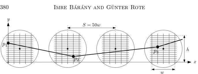
a horizontal line which form part of an array of 2n consecutive grid points. We want to perturb them into convex position. If the faces of the embedding have at most k sides, then K ≤ k. It is more convenient to work with a rectangular grid. So we extend the hexagonal grid to a rectangular grid as shown in Figure 9. This grid will be refined sufficiently in order to allow a strictly convex chain to be drawn inside a sequence of circles. Figure 10 gives a schematic picture of the situation. (This drawing is not to scale.) It is more convenient to discuss the construction of anupward convex chain. Inside each disk (of radius 1/30) we fit a square of side length 1/50, which is subdivided into a subgrid of width w and height h. More precisely, we are looking for a sequence of pointspi= (xi, yi) in these circles, whose coordinates measure the
distance from the lower left corner of the first circle in units of little grid cells. Two successive circle centers at distance 1 in terms of the original grid have a distance of S := 50wwhen measured in subgrid units. Thus we are looking for integer coordinates that satisfy ai·S ≤ xi ≤ai·S+w and 0≤yi ≤ h.
Eventually, when the whole subgrid is scaled to the standard grid Z×Z, xi
andyi will become true distances again. The total size of the resulting integer
grid will be O(nw)×O(nh).
The convex chainp1, p2, . . . , pK has a descending part up to a point with
min-imum y-coordinate and an ascending part. We choose the two points with minimum y-coordinate to lie in the middle: We define M :=⌊K/2⌋+ 1 and set yM−1 =yM = 0. We will only describe the construction of the ascending
chain frompM to the right. The left half is constructed symmetrically.
The direction between two grid points is uniquely specified by aprimitive vec-tor, a vector whose components are relatively prime. We now take a sequence of primitive vectorsq1, q2, . . . , qK−M,qi= (ui, vi) with 0< ui≤wandvi>0,
in order of increasing slopevi/ui. Then we choose the difference vectors ∆pas
p2
p3 p1
w
h
S= 50w
y
x
Figure 10: A convex chain formed by grid points in the circles. (Again, the radius of the circles is drawn much too large compared to their distance.)
definedyM := 0, and we choosexM arbitrarily within the permitted range of
x-coordinates. Having definedpM+i−1, we define
pM+i:=pM+i−1+s·qi
by adding as many copies ofqias are necessary to bringxM+iinto the desired
box:
aM+i·S≤xM+i≤aM+i·S+w
Since this box has widthw, andui≤w, this is always possible.
We need K−M ≤K/2 primitive vectors qi (including the vector (1,0) from
pM−1topM.) The following theorem ensures that we can find these vectors in
a triangle of sufficiently large area.
Theorem 2. The right triangleT = (0,0),(w,0),(w, t), wherew≥1,w inte-ger, andt≥2, contains at leastwt/4 primitive vectors.
The general proof is given in Section 5. We can however easily give an explicit solution for the special case t= 2 (corresponding to the choice w=k below, which leads to the most balanced grid dimensions): In this case, we can simply take the 1 +⌊w/2⌋vectors (w,1), (w−1,1), . . . , (⌈w/2⌉,1).
We use Theorem 2 as follows. We choose an arbitrary width w ≤ k for the boxes. By Theorem 2, we can set t := max{2,2K/w} to ensure that we find at leastK/2 primitive vectors in the triangle T. The slope of these vectors is bounded by t/w. Let us estimate the necessary height h of the boxes. The last pointpK is connected topM by a chain of vectors with slope at mostt/w.
The distance ofx-coordinates is at most the width of the whole grid on which the graph is embedded, i. e., at most S·2n = O(wn); hence the difference in y-coordinates is at most t/w·O(wn) =O(tn) =O(kn/w). It follows that the heighthof the boxes isO(kn/w). The total height of the resulting grid is O(hn) =O(kn2/w).
(a) (b) (c)
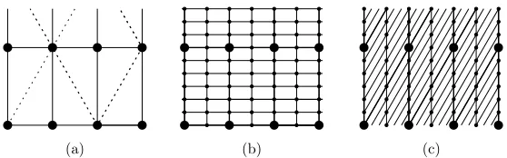
Figure 11: A rectangular grid (a), its 2×6 refinement (b), and a shearing (c) of the refined grid. Its grid-points coincide with the untransformed grid.
4.3 Perturbation of Vertices on Diagonal Lines
So far, we have treated only a sequence of vertices on a horizontal straight line. The same scheme can be applied to lines of the two other directions by applying the shearing transformation¡x
y
¢
7→¡ x y+√3/2·x
¢ or¡x
y
¢
7→¡ x y−√3/2·x
¢
which moves points only in vertical direction. Ifhis a multiple ofw, the transformation will produce a grid like in Figure 11c which is contained in the original grid of Figure 11b. For the range of parameters which is interesting for the theorem (w≤k), the heighthof the subgrid is never smaller than the width w; thus, the choice of h as a multiple ofw does not change the asymptotic analysis. One needs to reduce the size of the little square subgrid to ensure that the sheared square still fits inside the circle, and one has to adjust the quantity S accordingly. In addition, we have to select h and w as multiples of 14, to accommodate the grid of the rough perturbation and the refined rectangular grid of Figure 9b. All of this changes the analysis only by a constant factor. For the case of a uniform stretching of both dimensions (w =h), one referee has pointed out a simpler alternative method. After a blow-up by a factor of two, the original triangular grid contains rectangular grids in all three grid directions, Figure 9c. Two further refinements by the factor 7 (for the rough perturbation) and then by the factorware sufficient to accommodate the fine perturbation. On the exterior edges, the points must of course be perturbed to form an outward convex chain.
For part (iii) of the theorem we have already mentioned that interior faces with k≤4 sides are already strictly convex. If the outer face has 4 edges, it contains a single vertex on one of the sides of the outer triangle. The rough perturbation is thus sufficient to make the outer face strictly convex.
The whole procedure, as described above, is quite explicit and can be carried out with a linear number of arithmetic operations. We calculate the O(k) primitive vectors qi only once and store them in an array. Then, for every
optimal greedy
w=h n (w+ 1)/n n (w+ 1)/n
0 2 0.5000 2 0.5000
1 4 0.5000 4 0.5000
2 6 0.5000 6 0.5000
4 10 0.5000 8 0.6250
6 14 0.5000 12 0.5833
8 16 0.5625 14 0.6429
10 20 0.5500 18 0.6111
12 22 0.5909 18 0.7222
20 32 0.6562 28 0.7500
40 58 0.7069 48 0.8542
100 122 0.8279 96 1.0521
200 212 0.9481 164 1.2256
400 366 1.0956 276 1.4529
1,000 758 1.3206 562 1.7811
2,000 1,292 1.5488 948 2.1108 4,000 2,206 1.8137 1,610 2.4851 10,000 4,468 2.2384 3,230 3.0963 20,000 7,592 2.6345 5,472 3.6552
40,000 9,250 4.3244
100,000 18,484 5.4101
200,000 31,192 6.4119
400,000 52,626 7.6008
1,000,000 105,012 9.5227
2,000,000 177,046 11.2965
4,000,000 299,494 13.3559
Table 1: The length of the longest strictly convexn-gon in a sequence of square cells of sizew×w, regularly spaced at distanceS= 50w.
4.4 Numerical Experiments
We have presented a general systematic solution for finding a convex chain by selecting grid-points from a sequence of boxes. One can find the optimal
(i.e., longest) convex chain in polynomial time by dynamic programming, as described in more detail below. Results of some experiments are shown in the first column of Table 1. We restrict ourselves to the standard situation of selecting ann-gon fromnadjacent boxes (K=n) which are squares (w=h). For several different sizes w, we computed the largest n such that a strictly convex n-gon can be found in a sequence of cells of size w×w. The factor (w+1)/ndetermines the necessary grid sizewin terms ofn. (By the convention of Figure 10, a “w×w” grid consists of (w+1)2vertices; thus we give the fraction
decreasing and a monotone increasing part, connected by a horizontal segment in the middle, the necessary height w+ 1 is at least 0.5n. We see that this trivial lower bound is achieved for small values of n. The factor (w+ 1)/n increases with n, but not very fast. (The rectangularw×hboxes constructed in the proof of Theorem 1 would havew/n= 1, buth/n= 100.)
The dynamic programming algorithm computes, for each pointpin thew×h box, and for each possible previous pointp′ in the adjacent box to the left, the longest ascending and strictly convex chain (of length i) for which pi−1 = p′
and pi =p. Knowing p′ andp, it can be determined which points in the next
box are candidate endpointspi+1of a chain of lengthi+1. One can argue that,
among these points pi+1 that are reachable as a continuation ofp′p, only the
w+ 1 lowest points on each vertical line are candidates for endpointspi+1that
form part of an optimal chain. Theoretically, the complexity of this algorithm is thereforeO(w3h2). It turns out that, with few exceptions, every pointphas
only one predecessor point p′ that must be considered: all other predecessor pointspi−1have either a larger slope of the vectorp−pi−1or they are reached
by a shorter chain. Therefore, the algorithm runs inO(w2h) =O(wkn) time,
in practice.
A simple greedy approach for selecting the points pi one by one gives already
a very good solution: we choose pi+1 from the possible grid points in the
appropriate box in such a way that the segmentpi+1−pihas the slope as small
as possible while still forming a convex angle at pi. The results in the right
column of Table 1 indicate that this algorithm is quite competitive with the optimum solution. The running time is O(kw).
5 Grid Points in a Triangle
In this section we prove Theorem 2. We denote byP:={(x, y)|gcd(x, y) = 1} the set of primitive vectors in the plane.
It is known that the proportion of primitive vectors among the integer vectors in some large enough area is approximately 1/ζ(2) = 6/π2 [10, Chapters 16–
18]. Thus, a “large” triangle T should contain roughly 3/π2
·wt ≈ 0.304wt primitive points. However, for very wide or very high triangles, the fraction of primitive vectors may be different. In fact, fort= 2, the boundwt/4 is tight except for an additive slack of at most 2.
5.1 Fixed width, unbounded height
For a fixed value ofw, the functionf(t) :=|T∩P| can be analyzed explicitly. It is periodically ascending:
f(t+w) =f(t) +C,
where C=Pw
i=1φ(i) is the number of primitive vectors in the triangle (0,0),
(w,0), (w, w), excluding the point (1,1). Euler’s totient function φ(i) denotes the number of integers 1≤j≤ithat are relatively prime toi, or equivalently, the number of primitive vectors (i, j) on the vertical line segment from (i,0) to (i, i−1).
The reason for the periodic behavior is that the unimodular shearing transfor-mation (x, y)7→(x, y+x) maps the triangle (0,0), (w,0), (w, t), to the triangle (0,0), (w, w), (w, w+t), which is equal to (0,0), (w,0), (w, w+t) minus the triangle (0,0), (w,0), (w, w).
Therefore, it is sufficient to check that the “average slope”C/woff is bigger thanw/4, and to check
f(t)≥tw/4 (1)
for the initial interval 2≤t≤2 +w. This can be done by computer: We sort all primitive vectors (x, y) with 0≤x≤wand 0≤y/x≤(w+ 2)/w by their slopey/x. We gradually increasetfrom 2 tow+ 2. The critical values oft for which (1) must be checked explicitly are when a new primitive vector is just about to enter the triangle.
We ran a lengthy computer check to establish (1) for w= 1,2, . . . ,250 and for 2 ≤t ≤w+ 2 (and hence for all t). In addition, we checked it for the range w= 251,252, . . . ,800 and for 2≤t≤250.
5.2 Large width
In this section we prove Theorem 2 for small t and large w. T intersects each horizontal line y =i in a segment of lengthw−(w/t)i. In any set ofi consecutive grid points on this line, there are preciselyφ(i) primitive vectors. We can subdivide the grid points ony=iinto⌊(w−(w/t)i)/i⌋ ≥w/i−w/t−1 groups oficonsecutive points, leading to a total of at least (w/i−w/t−1)φ(i) primitive vectors:
For a given value of⌊t⌋, one can evaluate the expression
explicitly. The right-hand side of this bound is a linear function g(w): g(w)> w·131/4> wt/4 forw≥762. Performing this calculation by computer for ⌊t⌋ = 6,7, . . . ,130 establishes Theorem 2 for 6 ≤ t ≤ 130 and w ≥ 800.
counting the primitive vectors on the linesy= 0,y= 1, andy= 2, respectively. Fort≥3, the right-hand side of (3) is still valid as a lower bound. We get
|T∩P| ≥1 +¡
whose right angle lies on a grid point. Then
areaT′ ≤ |T′∩Z2| ≤areaT′+⌊a′⌋+⌊b′⌋+ 1
a′
b′
a
b y
x
T∗
T (a)
(b)
T′
Figure 12: (a) The triangle T′ in Lemma 3 and its covering by squares. (b) The triangles T and T∗ (shaded) in Lemma 4.
Proof. See Figure 12b. The triangleT∗ has length a−a/b, height b−1 and area 1
2(b−1)(a−a/b) =ab/2−a+a/(2b). LetT′ denote the part ofT∗ that
lies left of the linex=⌊a⌋. This triangle contains the same grid points asT∗. We assume first thatT′ is a nonempty triangle. The difference in areas lies in a rectangle strip of width<1 and heightb−1:
areaT∗−(b−1)≤areaT′≤areaT∗
We can apply Lemma 3 toT′ and obtain
|T∗∩Z2|=|T′∩Z2| ≤³ab2 −a+ a 2b
´
+³a−a b ´
+ (b−1) + 1,
|T∗∩Z2|=|T′∩Z2| ≥areaT′ ≥³ab 2 −a+
a 2b
´
−(b−1),
from which the lemma follows.
The triangleT′may not exist, as in Figure 13. In this case,T∗∩Z2=
∅. Instead of arguing why the above derivation is valid also for this case, we establish the inequalities directly. Letb′≥b−b/adenote the vertical extent ofT atx=⌊a⌋. Then the fact thatT′ is empty is equivalent tob′ <1.
Then, from 1≥b′ ≥b−b/awe conclude thatab < a+b. It follows that the lower bound in (4) is at most 0:
ab 2 +
a
2b −a−b≤ a+b
2 +
a
2 −a−b≤0
a
Figure 13: If T∗ (shaded) contains no grid points, the triangle T′ does not exist.
The number of primitive vectors can be estimated by an inclusion-exclusion formula, taking into account vectors which are multiples of single primes 2,3,5,7, . . ., vectors which are jointly multiples of two primes, of three primes, and so on, see [10, Chapters 16–18]:
|T∩P|= 1 +|T∗∩P|= 1 +
leading to the fact mentioned above that a fraction of approximately 6/π2 of
the grid points in a large area are primitive vectors.
Our sum in (5) goes to i = ∞, but for i > w or i > t, the set (1iT)∗ ∩Z2
whereHS = 1+1/2+1/3+· · ·+1/Sis the harmonic number. The last inequality
comes from bounding the remainder P∞
i=S+1µ(i)/i2 ≤
P∞
i=S+11/i2<1/Sof
the infinite series, whose value is 6/π2.
Combining the two cases and settingn:= min{w, t} gives
|T∩P| ≥wt µ 3
π2 −
1 2(n−1) −
2H⌊n⌋ n
Using the estimate Hi ≤γ+ ln(i+ 1) with Euler’s constant γ ≈0.57721, it
can be checked that this factor is bigger than 1/4 for n≥ 250, thus proving the theorem forw, t≥250.
On the other hand, the factor in (6) is bigger than 1/4 for w ≥ 800 and 130≤t≤250, proving the theorem also for this range.
Wrap-up. The proof of Theorem 2 is now complete. On a high level, we distinguish three ranges for w: 1≤w≤250, 251≤w≤800, andw≥800.
• Range 1: For 1 ≤ w ≤ 250, the theorem has been established in Sec-tion 5.1.
• Range 2: 251 ≤ w ≤ 800. For 251 ≤ w ≤ 800 and 1 ≤ t ≤ 250, the theorem has been established in Section 5.1 as well. For 251≤w≤800 andt≥250, it has been proved in Section 5.3.
• Range 3: Finally, forw ≥800, there is a division into three cases: Sec-tion 5.2 takes care of the range 2≤t≤130. Section 5.3 proves the bound separately for the ranges 130≤t <250 andt≥250.
6 Conclusion
In practice, the algorithm behaves much better than indicated by the rough worst-case bounds that we have proved. We have not attempted to optimize the constants in the proof. For example, if we don’t take a 7×7 subgrid but an 11×11 subgrid, and with a more specialized treatment of the outer face, the permissible amount of perturbation in Lemma 1 increases from 1/30 to 1/9, but it would make the pictures of the rough perturbation harder to draw. Bonichon, Felsner, and Mosbah [4] have used a technique of eliminating edges from the drawing that can later be inserted in order to reduce the necessary grid size for (non-strictly) convex drawings. This technique can also be applied in our case: remove interior edges as long as the graph remains three-connected. These edges can be easily reinserted in the end, after all faces are strictly con-vex. (For non-strictly convex drawings in [4], the selection of removable edges and their reinsertion is actually a more complicated issue.) This technique might be useful in practice for reducing the grid size.
In contrast, the faces that are produced in our algorithm have a very restricted shape: when viewed from a distance, the look like the triangles, quadrilaterals, pentagons, or hexagons of then×ngrid drawing from which they were derived. To reduce the area requirement below O(n4) one has to come up with a new
approach that also produces faces with a “rounder” shape.
Our bounds are however, optimal within the restricted class of algorithms that start with a Schnyder drawing or an arbitrary non-strictly convex drawing on anO(n)×O(n) grid and try to make it strictly convex by local perturbations
only. Consider the case wheren−1 vertices lie on the outer face, connected to a central vertex in the middle. The Schnyder drawing will place these vertices on the enclosing triangle, and at least n/3 vertices will lie on a common line. They have to be perturbed into convex position, as in Figures 7 or 10. Let us focus on the standard situation when we want to perturbnequidistant vertices on a line, at distance 1 from each other. Then−1 edge vectorspi+1−pi
lie in a 2w×2hbox; they must be non-parallel, and in particular, they must be distinct. If ∆y is the average absolute vertical increment of these vectors, it follows that ∆y= Ω(n/w), and the total necessary heighthof the boxes is Ω(n(∆y)) = Ω(n2/w). Therefore, the total necessary area is Ω(hwn2) = Ω(n4).
The argument can be extended to the case when only Ω(n) selected grid vertices on a line of lengthO(n) have to be perturbed. It can also be shown that our bounds in terms ofk are optimal in this setting. The worst case occurs when there is a line of lengthnwith Ω(k) consecutive grid points in the middle and two vertices at the extremes.
Extensions. The class of three-connected graphs is not the most general class of graphs which allow strictly convex embeddings. The simplest example of this is a single cycle. A planar graph, with a specified face cycle C as the outer boundary, has a strictly convex embedding if and only if it is three-connected to the boundary, i. e., if every interior vertex (not onC) has three vertex-disjoint paths to the boundary cycle. Equivalently, the graph becomes three-connected after adding a new vertex and connecting it to every vertex of C. These graphs cannot be treated directly by our approach, since the Schnyder embedding method of Felsner [8] does not apply. Partitioning the graph into three-connected components and putting them together at the end might work.
Acknowledgements. We thank the referees for helpful remarks which have lead to many clarifications in the presentation. Imre B´ar´any was partially supported by Hungarian National Science Foundation Grants No. T 037846 and T 046246.
References
inteligencia1 (1982), no. 6, 549–558.
[2] , On the maximal number of edges of convex digital polygons in-cluded into an m×m-grid, J. Comb. Theory, Ser. A69(1995), 358–368. [3] Imre B´ar´any and Norihide Tokushige,The minimum area of convex lattice
n-gons, Combinatorica24(2004), no. 2, 171–185.
[4] Nicolas Bonichon, Stefan Felsner, and Mohamed Mosbah,Convex drawings of 3-connected plane graphs, Graph Drawing: Proc. 12th International Symposium on Graph Drawing (GD 2004), September 29–October 2, 2004 (New York), J´anos Pach, ed. Lecture Notes in Computer Science, vol. 3383, Springer-Verlag, 2005, pp. 60–70.
[5] M. Chrobak and G. Kant, Convex grid drawings of 3-connected planar graphs, Internat. J. Comput. Geom. Appl.7 (1997), no. 3, 211–223. [6] Marek Chrobak, Michael T. Goodrich, and Roberto Tamassia, Convex
drawings of graphs in two and three dimensions, Proc. 12th Ann. Sympos. Comput. Geom., 1996, pp. 319–328.
[7] H. de Fraysseix, J. Pach, and R. Pollack,How to draw a planar graph on a grid, Combinatorica10(1990), no. 1, 41–51.
[8] Stefan Felsner,Convex drawings of planar graphs and the order dimension of 3-polytopes, Order18(2001), 19–37.
[9] , Geodesic embeddings and planar graphs, Order 20(2003), 135– 150.
[10] G. H. Hardy and E. M. Wright,An Introduction to the Theory of Numbers, Oxford Science Publications, 1979.
[11] J¨urgen Richter-Gebert,Realization Spaces of Polytopes, Lecture Notes in Mathematics, vol. 1643, Springer-Verlag, 1997.
[12] G¨unter Rote,Strictly convex drawings of planar graphs, Proceedings of the 16th Annual ACM-SIAM Symposium on Discrete Algorithms (SODA), Vancouver, 2005, pp. 728–734.
[13] W. Schnyder,Embedding planar graphs on the grid, Proc. 1st ACM-SIAM Sympos. Discrete Algorithms, 1990, pp. 138–148.
[14] W. Schnyder and W. T. Trotter,Convex embeddings of 3-connected plane graphs, Abstracts of the AMS13(1992), no. 5, 502.
[15] W. T. Tutte,Convex representations of graphs, Proceedings London Math-ematical Society10(1960), no. 38, 304–320.
Imre B´ar´any R´enyi Institute
Hungarian Academy of Sciences PoB 127
Budapest 1364, Hungary [email protected]
and
Department of Mathematics University College London Gower Street
London WC1E 6BT, UK
G¨unter Rote
Freie Universit¨at Berlin Institut f¨ur Informatik Takustraße 9