M – 22 PRICE OF SUGAR MODELING AND FORECASTING BASED ON
STIMA MODEL AND GSTIMA MODEL
Dania Siregar, M. Nur Aidi, I Made Sumertajaya Statistics Department, FMIPA, Institut Pertanian Bogor
Abstract
STIMA (space-time integrated moving average) model is a special form of Vector IMA model that combines the interdependence of time and location that is known by space-time model. STIMA model requires the same parameter values for all locations, so Generalized-STIMA (GSTIMA) model is developed to overcome this problem. This paper compares the implementation of two models in forecasting the price of sugar in capital provinces in Sumatra Island, Indonesia. The first step is model building for each model. This step is similar to Box-Jenkins’s procedure. It is begun with the determination of temporal order by using AICC, while spatial order is restricted on order 1, the parameter estimation uses nonlinear least square method that are minimized by a Gauss-Newton algorithm, and then diagnostic checking of white noise errors. The normalization of cross-correlation between the locations at the appropriate time lag is used as space weight. The last, the implementation of forecastis evaluated by using the Root Mean Square Error (RMSE) where the error is defined as the differences between the actual value and the forecastvalue. The implementation of STIMA model is better compared with GSTIMA model in forecasting the price of sugar, although STIMA model produces the same parameters for each location.
Key words: Space-time, STIMA, GSTIMA, Modeling, Forecasting.
INTRODUCTION
The data of multivariate time series can be modeled with VARMA model (Vector Autoregressive Moving Average) which is an extension of the ARMA model. A special form of VARMA model is STARMA (Space-Time Autoregressive Moving Average) model which combines the interdependence of time and location. This model was first introduced by Pfeifer and Deutsch (1980). However, STARMA model is sometimes considered unrealistic because the parameters are assumed equal for all locations. This assumption is considered not to have a strong theoretical basis and less able to accommodate heterogeneity locations. Borovkova et al. (2002) proposed that GSTARMA (Generalized Space-Time Autoregressive Moving Average) model also can combine the interdependence of time and location. This model is considered more realistic because it produces different parameters for each location. The STARMA model and GSTARMA model with zero order for MA and with applying first difference can be called STIMA model and GSTIMA model.
the strategic commodities in Indonesian economy. The forecast of sugar price will be very useful for designing the system that will be built both by the government or the food and beverage industry.
This research will make the models for the phenomenon of sugar price in eight capital provinces in Sumatra Island by using GSTIMA and STIMA model. GSTIMA model is considered more theoretical and complex rather than STIMA model. However, it still becomes a separated question, whether the GSTIMA model is better than STIMA model to forecast the sugar price in the capital provinces in Sumatra. This study will examine the comparison of the models and the implementation of forecasting models in modeling and forecasting sugar price by using the normalized cross-correlation as space weight.
RESEARCH METHOD Method and Material
This research is a comparative study of STIMA and GSTIMA model in forecasting sugar price in eight capital provinces in Sumatra island, namely, Banda Aceh, Medan, Padang, Pekanbaru, Bengkulu, Jambi, Palembang and Bandar Lampung. Sumatra island was chosen as the subject of the research because Sumatra island is included the second largest island in producing sugar after Java island, and also has larger area than Java island. Sugar-producing provinces in Sumatra island are Lampung, South Sumatra and North Sumatra. And the other provinces are not sugar-producing provinces. The effect of spatial interaction which relates to the phenomenon of inter-provincial sugar price can be seen from the influence of sugar distribution, transportation and production costs. Besides, sugar is included as food products which is controlled and regulated by the government because it has the effects toward the national economy and becomes one of the indicators in inflation measurement.
The data used in this research was secondary data. It was the time series data of sugar price in eight capital provinces in Sumatera Island. The time series data was weekly price (288 series) which was obtained from the average daily per week in the beginning of January 2008 until December 2013. The procedure obtained that STIMA and GSTIMA model were done with the help of MINITAB and SAS program through the steps of identification of time and spatial order, the formation of normalization cross-correlation weight matrix, parameter estimation, diagnostic checking, until the forecast. After getting the forecasts of two models, it was followed by doing the comparison of implementation forecasting between two models by comparing RSME value. The smaller RSME value, the better implementation of model in forecasting.
Methodology
Vector ARIMA Model
For example, = [ , , ,, …, , ]′, = 0, 1, 2, … , with m-dimensional, where
is a series of sugar price that is not stationary, then the model VARIMA order p, d, q is defined, as follows (Wei 1990):
( ) ( ) = ( ) ( 1) where ( ) = − − − ⋯ −
( ) = − − − ⋯ −
and are nonsingular matrix sized × , with assume = =
and ( ) =
⎣ ⎢ ⎢
⎡( 1− ) 0 ⋯ 0
0 ( 1− ) ⋱ ⋮
⋮ ⋱ ⋱ 0
0 ⋯ 0 ( 1− ) ⎦⎥
⎥ ⎤
The shift backward of operator B and its use as follows = , and ( 1− ) = , so that when q = 0 then becomes a model VARI (p) can be written in the form
And when p = 0 then becomes a model VIMA (q) can be written in the form
= − − + ⋯ − ( 3)
Space-Time IMA Model
STIMA model is an extension of VIMA model which has been modified with the main differences in adding the weight of matrix location. STARIMA Model is defined as follows:
= − θ ( ) + , ( 4)
with [ ] = and , ′ = , = 0
, ℎ
where shows the kth spatial order of the moving average, θ is the parameter of moving average on the kth time lag and the lth spatial lag, and ( ) is an m × m matrix of spatial weight for the spatial order l which has a zero diagonal.
Generalized Space-Time IMA Model
Generalized Space-Time Model was proposed by Borovkova et al. (2002), GSTIMA is a development of the STIMA model. In STIMA model parameters are assumed equal for each location. This assumption makes STIMA model simpler because it has fewer parameters. However, this assumption makes STIMA is considered inflexible and unrealistic in describing the characteristics of the location which is probably not homogeneous. The fundamental differences of two models is on the parameters, which in the model STIMA θ are constant, while in GSTIMA model the form are matrix of . It causes GSTIMA more difficult in the calculation parameters. GSTIMA model is defined as follows:
= − ( ) + , ( 5)
where,
= (θ ( ), …,θ ( ) =
θ ( )
, 0 0
0 ⋱ 0
0 0 θ ( )
Model Identification
As in time series modeling, the first step is identifying a tentative model which is characterized by spatial and time order. Spatial order is restricted on order 1, because the higher order is difficult to be interpreted (Wutsqa et al., 2010). Approving the method in VARMA model, the time order is determining by using the Akaike Information Corrected Criterion (AICC). The identification of time order is done by doing AICC value.
= log
~
+ 2
( − ) / ( 6)
Where ∑~ = ∑ ′ is matrix of the maximum estimator for the covariance of residual of the model, k is the number of variables, r is the number of estimated parameters and T is the number of observations.
Determination of Space Weight
The determination of space weight by using the normalization result of cross-correlation between locations at the appropriate time lag was firstly proposed by Suhartono and Atok (2006) in Suhartono and Subanar (2006). In general, the cross-correlation between the location of the ith and jth on the all time lag k, [ ( ) , ( − ) ] is defined as
where ( ) is the cross covariance between the observations in the location of the ith and jth location in the kth time lag, and are the standard deviation of the observations in the location of the ith and jth location. The estimation of the cross-correlation in the data sample as follows:
( ) = ∑ [ ( ) − ] [ ( − ) − ]
[ (∑ [ ( )− ] ) (∑ [ ( )− ] ) ] / . ( 8)
Furthermore, the determination of the weight matrix can be solved by normalizing the cross-correlation between the locations at the appropriate lag. This process generally produces weight location as follows
= | ( ) |
∑ ( ) , where ≠ , = 0, 1, 2 …, ( 9)
and satisfies ∑ = 1.
Parameter estimation
Parameter estimation for models of STIMA and GSTIMA can be done by minimizing the squared residual
= ( )′ ( ) ( 10) where ( ) for GSTIMA model with , = 0,1, . . ,
= + ( ) . ( 11) the same way is also used for STIMA model. However, the presence of the moving average component equation, then S becomes nonlinear so that S can be minimized by using the
Gauss-Newton algorithm (Zhou & Buongiorno, 2006).
Diagnostic Checking
To determine the constructed models has a decent former for forecasting. It is necessary to check whether the residuals of the model are approximately white noise, which means that the effective information of sugar prices has been exploited effectively by the model. If the autocorrelation decline zero in almost all lags , it means that the residuals are uncorrelated and the residuals close to white noise and STIMA and GSTIMA model construction are available (Min et al., 2010).
RESULT AND DISCUSSION Preliminary Model Building
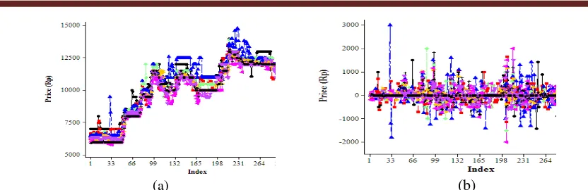
This modeling requires stationary process in data, so that in the first step is checked the stationary of data. The plot of sugar price time series data for each capital city can be seen in Figure 1(a). It shows that the data does not stationary in mean. Therefore, to achieve the stationary data, the first difference transformation must be applied. ( ) represents the sugar price for capital city i, i=1,2,..,8 at time t, t=1,…,288. The first difference transformation of
( ) denoted by ( ) is
(a) (b)
Figure 1 (a) The data of the original sugar prices in 8 capitals in Sumatera island and (b) The data of the original sugar prices after applied the first difference.
After the data meets the assumptions of stationary. For the purpose of forecasting, the data is grouped into the training data set and test data set. The training data are 268 data observations that will be used for model and the test data are the last 20 data that will be used in comparison of the implementation forecasting.
STIMA and GSTIMA Model Building for the Sugar Price Data
Determination of Space Weight
The weight normalized cross correlation does not require specific rules, such as depending on the distance between locations. In this research, the cross-correlation sugar price among locations can be weight with the principle of the greater cross-correlation, the greater weight given. The results of normalization cross-correlation between the locations at the appropriate lag for this case can be seen in Figure 2 and Figure 3.
Figure 2 The cross-correlation matrix between the location at the lag temporal 1
Figure 3 The cross-correlation matrix between the location at the lag temporal 2
Model Identification
because the higher order is difficult to be interpreted (Wutsqa et al., 2010). Table 1 shows that the smallest value of AICC is MA model order 2. Thus, the models that will be built are STARIMA and GSTARIMA models with the order of temporal AR (0), MA (2) and spatial order 1 with first difference. This model is called as STIMA and GSTIMA model.
Table 1 Minimum Information of Criterion Based on AICC
Lag MA 0 MA 1 MA 2 MA 3 MA 4 MA 5
AR 0 88.370943 88.195071 88.047394 88.312579 88.577849 88.76531
AR 1 88.197916 88.321777 88.19572 88.486506 88.7942 89.092439
AR 2 88.085791 88.260814 88.444165 88.750117 89.201891 89.471196
AR 3 88.349011 88.545572 88.741617 89.152278 89.529882 89.76491
Parameter Estimation
The results of parameter estimation for STIMA and GSTIMA model with the temporal order MA (2), spatial order 1 can be seen in Table 2 and Table 3. GSTIMA model produces more parameters than STIMA model, so that GSTIMA model is more complex than STIMA model.
Table 2 The estimation of nonlinear OLS for STIMA parameter
Parameter Estimate t-value Approx Pr > |t|
θ -0.210 -9.34 <.0001*
θ 0.501 15.27 <.0001*
θ -0.244 -10.68 <.0001*
θ 0.233 6.88 <.0001*
*significant at alpha 5%
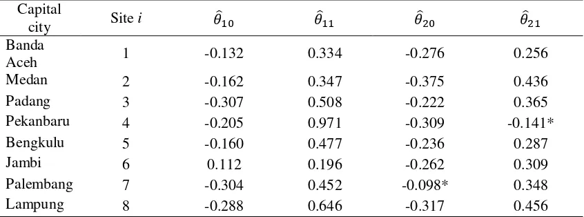
Table 3 The estimation of nonlinear OLS for GSTIMA parameter Capital
city Site i Banda
Aceh 1 -0.132 0.334 -0.276 0.256
Medan 2 -0.162 0.347 -0.375 0.436
Padang 3 -0.307 0.508 -0.222 0.365
Pekanbaru 4 -0.205 0.971 -0.309 -0.141*
Bengkulu 5 -0.160 0.477 -0.236 0.287
Jambi 6 0.112 0.196 -0.262 0.309
Palembang 7 -0.304 0.452 -0.098* 0.348
Lampung 8 -0.288 0.646 -0.317 0.456
*insignificant at alpha 5%
+ ( ) ( 13)
and based on Table 3, GSTIMA model for location i, i= 1,2, …, 8 as follows
( ) = − θ( ) ( −1) −θ( ) ( −1) −θ( ) ( −2) −θ( ) ( −2)
+ ( ) ( 14)
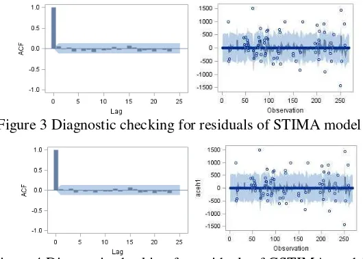
Diagnostic Checking
To determine the constructed models has a decent former for forecasting. It is necessary to check whether the residuals of the model are approximately white noise, which means that the effective information of sugar prices has been exploited effectively by the models. The result of diagnostic checking for each capital city is good because autocorrelation decline almost zero in the all lags. Therefore, the residuals close to white noise and the models we just build are available. For example, Figure 3 and Figure 4 are two autocorrelation function (ACF) graph for STIMA and GSTIMA models in Aceh capital city. In the figures, it is evident that the residuals of STIMA and GSTIMA models are close to the white noises. The mean of the residuals is nearly zero and the ACF graph shows that ACF decline rapidly after order 0 and insignificant at almost all lags, which indicates that the residuals are uncorrelated and the residuals close to white noise and STIMA and GSTIMA model construction are available.
Figure 3 Diagnostic checking for residuals of STIMA model
Figure 4 Diagnostic checking for residuals of GSTIMA model
Comparative Study
For the purpose of forecast, the estimated parameters in Table 2 for STIMA model and space weight from Figure 2 and Figure 3 can be used to forecast the h-step-ahead prediction value, as follows:
( + ℎ)
= − θ ( −1 + ℎ) −θ ( −1 + ℎ)
−θ ( −2 + ℎ)−θ ( −2 + ℎ)+ (
+ ℎ) ( 15)
( + 1) = − ( ) − ( )− ( −1)
− ( −1) + ( + 1) + ( ) .
( + 1) = − ( )− ( )− ( −1)− ( −1)
+ ( ) .
The value of ( + ℎ) will not be known because the expected value for random error in the future must be set equal to zero. However, from the fitted models we can replace the value ( ) , ( −1) , …, ( − ) with their value that is defined empirically, i.e. as obtained after the last iteration Gauss-Newton algorithm.
The 2-step-ahead prediction value, as follows:
( + 2) = − ( + 1)− ( + 1) − ( )
− ( ) + ( + 2) + ( + 1) .
( + 2) = − ( )− ( ) + ( + 1) .
The 3-step-ahead prediction value, as follows:
( + 3) = − ( + 2)− ( + 2) − ( + 1)
− ( + 1) + ( + 3) + ( + 2) .
( + 3) = ( + 2) .
The 4-step-ahead prediction value, as follows:
( + 4) = − ( + 3)− ( + 3) − ( + 2)
− ( + 2) + ( + 4) + ( + 3) .
( + 4) = ( + 3) .
Therefore, starting from 2-step-ahead prediction value until 20-step-ahead prediction value, the value of prediction is constant.
The estimated parameters in Table 3 for GSTIMA model and space weight from Figure 2 and Figure 3 also can be used to predict the h-step-ahead prediction value by using the same method as STIMA model above. The difference is only on the different parameters for each location, as follows:
( + ℎ) = −θ( ) ( −1 + ℎ)−θ( ) ( −1 + ℎ)−θ( ) ( −2 + ℎ)
−θ( ) ( −2 + ℎ) + ( + ℎ)
capitals in Sumatra island. Furthermore, the step is to compare two models of the implementation forecasting by using the Root Mean Square Error (RMSE) which is also called the Root Mean Square Deviation (RMSD). The RMSE is a measure that is frequently used of the difference between the values that is predicted by a model and the values that is observed from the environment that is being modelled. These individual differences are also called residuals, and the RMSE serves to combine them into a single measure of predictive power.
= ( 17)
where m many locations
= [ ( + ) − ( + ) ]
/
, ( 18)
To d is the size of the data used for testing the model with j=1,2, … ,20, and T is the size of modeled data that is 268 observations.
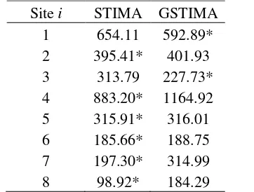
Table 4 The value of RMSE for each capital
Site i STIMA GSTIMA
1 654.11 592.89*
2 395.41* 401.93
3 313.79 227.73*
4 883.20* 1164.92
5 315.91* 316.01
6 185.66* 188.75
7 197.30* 314.99
8 98.92* 184.29
* The best implementation of forecasting
Table 4 shows the smallest RMSE value is more owned by STIMA model for each location, while by using the formula [17] obtained the results of RSME for STIMA and GSTIMA respectively about 380.54 and 423.94. The value of the average of RMSE from STIMA model is smaller than GSTIMA model. It can be concluded that the implementation of STIMA model forecasting is better than GSTIMA model for the forecasting of sugar price in eight capitals in Sumatra island.
CONCLUSION AND SUGGESTION
REFERENCES
Borovkova, S.A., Lopuhaa, H.P., & Nurani, B. (2002). Generalized STAR model with experimental weights. in: M Stasinopoulos & G Touloumi. Editor. Proceedings of the 17th International Workshop on Statistical Modeling. 139-147.
Min, X., Hu, J., & Zhang, Z. (2010). Urban Traffic Network Modeling and Short-term Traffic Flow Forecasting Based on GSTARIMA Model. 13th International IEEE, Annual Conference on Intelligent Transportation Systems; 2010 September 19-22; Madeira Island, Portugal,
Pfeifer, P.E., & Deutsch, SJ. (1980), A three stage iterative procedure for space-time modeling, Technometrics 22, 35-47.
Suhartono & Subanar. (2006). The Optimal Determination of Space Weight in GSTAR Model by using Cross-correlation Inference. Journal of Quantitative Methods: Journal Devoted to The Mathematical and Statistical Application in Various Fields, Vol. 2, No. 2, pp. 45-53.
Wei, W.(1990). Time series analysis: univariate and multivariate methods. New york: Addison-Wesley Publishing Co.
Wutsqa, D.U., Suhartono, & Sutijo, B. (2010). Generalized Space-Time Autoregressive Modeling. Proceedings of the 6th IMT-GT Conference on Mathematics, Statistics and its Applications (ICMSA2010); Kuala Lumpur, Malaysia.