Obesity, Weight Loss, and
Employment Prospects:
Evidence from a Randomized Trial
Arndt R. Reichert
Reichertabstract
This study presents credible estimates for the causal effect of BMI growth on employment among the obese. By exploring random assignment of a weight- loss intervention based on monetary rewards, I provide convincing evidence that weight loss positively affects the employment prospects of obese women but not of obese men. Consistent with this, signifi cant effects of weight loss on proxy variables for labor productivity are found only for obese women.
I. Introduction
Obesity rates are rapidly increasing in almost all industrialized coun-tries and in numerous emerging economies (for example, Prentice 2006). This is not only extremely worrisome for public health reasons but also from an economic perspective since obesity is found to turn Social Security contributors into welfare
Arndt R. Reichert is an economist at the World Bank and affi liated with the Rhine Westphalia Institute for Economic Research. He is grateful to Pakt für Forschung und Innovation for funding, Ronald Bachmann, Thomas K. Bauer, Hanna Frings, Mathilde Godard, Alfredo R. Paloyo, Sandra Schaffner, Christoph M. Schmidt, Hendrik Schmitz, Harald Tauchmann, Nicolas Ziebarth, and two anonymous reviewers for helpful comments. He also gratefully acknowledges the comments and suggestions of participants of the 23rd European Workshop on Econometrics and Health Economics, the German Health Economics Associa-tion meeting in 2012 and the European Conference on Health Economics 2012. He further acknowledges research assistance of Rüdiger Budde, Viktoria Frei, Karl- Heinz Herlitschke, Klaus Höhner, Julia Jochem, Mark Kerßenfi scher, Lionita Krepstakies, Claudia Lohkamp, Thomas Michael, Carina Mostert, Stephanie Nobis, Adam Pilny, Margarita Pivovarova, Gisela Schubert, and Marlies Tepaß. He wants to express his particular acknowledgements to the medical rehabilitation clinics of the German Pension Insurance of the federal state of Baden- Württemberg and the association of pharmacists of Baden- Württemberg for their support of and dedication to this experiment. In particular, he thanks Susan Eube, Michael Falentin, Ina Hofferberth, Marina Humburg, Silke Kohlenberg, Thomas Krohm, Max Lux, Tatjass Meier, Monika Reuss- Borst, Constanze Schaal, and Wolfgang Stiels. All views expressed in this paper should be considered those of the author alone and do not necessarily represent those of the World Bank. Access to the data used in this article can be obtained beginning January 2016 through December 2019 from Rüdiger Budde, Hohen-zollernstraße 1- 3, fdz@rwi- essen.de. Address for correspondence: Arndt R. Reichert, The World Bank, 1818 H Street, Washington, D.C. email: areichert@worldbank.de.
[Submitted April 2013; accepted May 2014]
ISSN 0022- 166X E- ISSN 1548- 8004 © 2015 by the Board of Regents of the University of Wisconsin System
The Journal of Human Resources 760
recipients. Several studies, for instance, show that the obese have a substantially lower employment probability than healthy- weight people (for example, Morris 2007; Han, Norton, and Stearns 2009). However, the evidence on the employment effects of obe-sity has not yet been settled.
There is an obvious diffi culty in establishing a causal relationship between obesity and employment because both states are most likely correlated with unobserved fac-tors. Unobserved time preferences, for example, are related to obesity through food consumption and physical activity as well as to employment through health capital investments. Another problem is that employment itself may affect body weight. One argument is that junk food is relatively cheap and, therefore, consumed more by unemployed relative to employed people. Recent studies have aimed to solve these identifi cation problems by employing instrumental variable (IV) estimation. However, concerns remain with respect to the validity of the employed instruments, such as the obesity status of biological relatives, because this may affect employment outcomes through other pathways like common household environmental factors (Lindeboom, Lundborg, and van der Klaauw 2010).
This study is the fi rst to use a randomized controlled source of variation in body weight to overcome potential reverse causality and endogeneity problems in the esti-mation of employment effects. The analysis is based on instrumental variables gener-ated in the course of a randomized experiment that was conducted with the primary purpose of examining the effectiveness of monetary rewards for weight loss. Obese medical rehabilitation patients were randomly assigned to a control group and two treatment groups, which were both fi nancially rewarded contingent on weight loss. As shown in Augurzky et al. (2012), the two rewards were very effective in motivat-ing the obese to lose weight,1 which qualifi es them as instrumental variables for the degree of obesity.
Compared to the instrumental variables that have been employed in the past, the signifi cant advantage of using the monetary rewards is that they are much less likely to operate on employment through channels other than body weight. The reasons are that they are, fi rst, uncorrelated with pre- intervention characteristics due to the experi-mental design and, second, they do not themselves alter employment preferences or other behaviors that may be relevant for employment.2 In relation to the second point, as related literature suggests (Charness and Gneezy 2009), the body weight impact of the monetary rewards is entirely attributable to their coupling with weight targets rather than effects of promised cash payments through anticipated additional income.3 In addition, monetary rewards at most only marginally alter the budget constraint of
1. There are further studies that provide evidence for the effectiveness of monetary rewards to induce indi-viduals to exhibit desired healthy behaviors (for example, Charness and Gneezy 2009; Augurzky, Reichert, and Schmidt 2012).
2. Keane (2010) presents an instructive discussion of the general problem of instrumental variables poten-tially affecting the response variable through channels other than the explanatory variable.
Reichert 761
participants—and therefore the labor- leisure tradeoff—because cash payments are realized after the intervention period. On this point, several studies have shown that individuals with liquidity constraints (such as the average study participant in this case) do not change contemporaneous consumption levels even if they anticipate posi-tive transitory income changes (for example, Jappelli and Pistaferri 2010, Beznoska and Ochmann 2012). This means that their behavior remains unaffected prior to the realization of these changes. In fact, I do not fi nd that the monetary rewards infl uence, for example, smoking and drinking behaviors or the likelihood to go on vacations dur-ing the intervention period. Hence, promised monetary rewards for weight loss should not, by themselves, alter the participants’ desire to work during the study period.
In contrast to previous studies on this topic, I examine the impact of weight change among individuals who, in great majority, remain obese during the studied time period rather than the impact of obesity per se. A further novelty of the study is the presenta-tion of separate estimates for the effects on the job- fi nding probability of obese unem-ployed and the probability of remaining emunem-ployed of obese employees for Europe’s largest economy. The latter effect has been less in focus although obese workers may have an increased risk of layoff or early retirement relative to healthy- weight workers.
The paper additionally presents estimates for the reduced- form effect, which cap-tures the causal impact of the weight- loss intervention on employment. It allows me to examine whether the intervention has direct benefi ts for the welfare system. Moreover, it enables me to be the fi rst to address the question of whether the employment pros-pects of the particular group of obese people may be improved by public intervention. If this turns out to be true, labor market programs explicitly designed for the obese would represent promising policy options and should include a fi nancial incentive scheme for weight loss. Finally, the paper helps to identify the appropriate target of labor market interventions. For the present study population, it is reasonable to assume that excessive weight and its associated problems represent the factors that most limit labor productivity and, by implication, employment prospects. Thus, in the case of obese individuals, interventions designed to combat overweight and obesity have the potential to outperform classical labor market programs such as training.
The Journal of Human Resources 762
that exhibits pronounced gender heterogeneity in reacting to weight loss is weight discrimination. Lack of data limits the possibility to explain in greater depth observed gender- specifi c heterogeneity in returns to weight loss.
The remainder of this paper is organized as follows. The subsequent section reviews the literature. Section III describes the experimental design and introduces the data, Section IV explains the estimation strategy, and Section V presents the estimation re-sults. Sections VI, VII, and VIII discuss the main fi ndings, and Section IX concludes.
II. Background
Obesity and, in turn, weight loss may affect employment prospects in vari-ous ways.4 An obvious argument for weight loss among the obese is the associated positive health effects.5 In fact, in a companion paper, Augurzky et al. (2012) fi nd some evidence of health improvements in the obese due to weight loss. These are likely to translate into an increase in working productivity (and a reduction in the risk of work incapacity). Another argument is that obese persons who successfully reduce their weight have consequently expanded the set of potential tasks and occupations with which they could be matched. For instance, Everett (1990) and Puhl and Brownell (2001) demonstrate that employers consider obese workers unfi t for public sales positions. Moreover, by losing weight, obese people signal a healthier lifestyle, which indicates that they are more willing to invest in human capital, implying expected improvements in future working productivity.6
Because weight loss represents a diffi cult task and often an important goal for the obese (Crawford, Jeffery, and French 2000), those who achieve it are likely to be more optimis-tic about achieving other goals, too. The improvement in self- confi dence may cause them to express their ideas in group meetings more often or to be more convincing in job inter-views.7 Recently, Mocan and Tekin (2011) provide evidence of the impact of self- esteem on wages. A similar argument is that they gain physical attractiveness, which was found to yield better employment prospects (for example, Hamermesh and Biddle 1994; Biddle and Hamermesh 1998). Mobius and Rosenblat (2006) connect the beauty premium with self- confi dence, fi nding that while physically attractive workers are more confi dent and better equipped with respect to oral skills, both attributes are causally related to higher wages. A further reason is that obese individuals who lose weight are likely to suffer less from labor market discrimination, which is an evident problem faced by the obese (Giel et al. 2012; O’Brien et al. 2012; Rooth 2009; Roehling, Roehling, and Pichler 2007).8
4. A model on the potential mediators of obesity on labor market outcomes is presented by Baum and Ford (2004) as well as by Bhattacharya and Bundorf (2009).
5. For instance, Wing et al. (2011) fi nd improvements in indicators of cardiovascular risk factors. Christensen et al. (2007) show that weight loss signifi cantly reduces physical disability in patients with knee osteoarthritis. Hooper et al. (2007) provide evidence for a decrease in painful musculoskeletal conditions. Brown, Goetz, and Hamera (2011) report mental health improvements in obese individuals with serious mental illness. Reviewing the literature, Blackburn (1995) confi rms positive health effects of weight loss.
6. For the importance of lifestyle for health, see Kenkel (1995) and Contoyannis and Jones (2004). 7. The huge importance of personality psychology in economics has been extensively shown (Bowles, Gintis, and Osborne 2001; Heckman and Rubinstein 2001; Borghans et al. 2008).
Reichert 763
The link between obesity and employment prospects has been extensively analyzed in the literature. While the majority of the studies focuses on the effect of obesity on wages (for example, Register and Williams 1990; Averett and Korenman 1996; Pagán and Dávila 1997; Cawley 2004; Baum and Ford 2004; Morris 2006; Bhattacharya and Bundorf 2009; Han, Norton, and Stearns 2009; Cawley, Han, and Norton 2009; Lund-borg, Nystedt, and Rooth 2010), there also exists an extensive literature on the effect of obesity on employment (for example, Morris 2007; Norton and Han 2008; Han, Norton, and Stearns 2009; Cawley, Han, and Norton 2009; Lindeboom, Lundborg, and van der Klaauw 2010; Caliendo and Lee 2013).
The majority of the studies have aimed to solve the endogeneity problem and re-verse causality by employing instrumental variable estimation.9 Here, the validity of the employed instrument is crucial for consistent identifi cation of the causal effect of interest. Cawley (2004) and Lindeboom, Lundborg, and van der Klaauw (2010) use the obesity status of biological relatives although the latter cast doubt on their suit-ability as instruments after extensive validity tests. Norton and Han (2008) employ genetic individual information linked to obesity. Yet, although some genes seem more and some seem less correlated with body weight, there is no “fat” gene or “skinny” gene (Norton and Han 2008). This implies that genes may also be correlated with sev-eral personality characteristics other than body weight. In turn, it has to be expected that they are correlated with unobservable variables such as further health risks, be-ing likely to affect employment through channels other than obesity and, hence, to confound the IV estimation (Wehby, Ohsfeldt, and Murray 2008; Lawlor et al. 2008; Lawlor, Windmeijer, and Smith 2008). Finally, Morris (2007) uses the prevalence of obesity in the area of residence that seems to be the most convincing approach. How-ever, despite extensively controlling for area characteristics, he is not able to rule out endogenous regional selection due to the cross- sectional nature of the data (see also Caliendo and Lee 2011).
So far, the empirical evidence has argued in favor of a negative effect of the body- mass index (BMI) (or being obese) on wages of women but not of men. Regarding the probability to be in employment, Morris (2007) reports a statistically signifi cant negative effect, which is smaller for men. Caliendo and Lee (2013) report a signifi cant effect only for women. Both analyses are based on data from continental European countries.10 Most of the papers that use U.S. data fi nd no effect of obesity on employ-ment. A plausible reason for the intercontinental discrepancy in the results may be a stronger wage rigidity in European countries that inhibit wages to adequately refl ect labor productivity differentials. This, in turn, would imply that the adjustment mecha-nism primarily works through the employment decision (Bertola, Blau, and Kahn 2001). In light of the critique on the employed instrumental variables and the ambigu-ity of the results, Lindeboom, Lundborg, and van der Klaauw (2010) state the need to “. . . analyze the corresponding effects in other countries, where the labor markets look different, and using different sources of variation in obesity.”
9. By using logistic regression and matching methods, Han, Norton, and Stearns (2009); Cawley, Han, and Norton (2009); and Caliendo and Lee (2013) make the critical assumption that all variables that affect the likelihood of being obese are accounted for in their analyses.
The Journal of Human Resources 764
III. Experiment and Data
The data were generated by a fi eld experiment, which is briefl y dis-cussed below. A more extensive discussion of the experiment is provided by Augurzky et al. (2012). The data set and descriptive statistics of the study population are subse-quently presented.
A. The Experiment
The experiment was carried out between March 2010 and January 2012. In total, 700 patients of four rehabilitation clinics in southwestern Germany were recruited for par-ticipation in the experiment. Two individuals had to be excluded from the trial because of pregnancy and cancer. For most patients of these clinics, medical rehabilitation is paid for by the German pension fund, which predominantly aims at avoiding unem-ployment or early retirement, requiring that the patient’s ability to work is generally recoverable. Therefore, a joint characteristic of the participating patients may be that, besides being obese, they were available for the labor market. Participants are het-erogeneous with respect to their health complaints. The clinic in Bad Kissingen spe-cializes in gastroenterology and endocrinology. Those in Bad Mergentheim and Isny primarily focus on orthopedics, whereas the clinic in Glottertal treats patients with psychosomatic disorders. Most of the participants are admitted on the basis of a diag-nosis other than adiposity. However, it often turns out that their symptoms are related to their weight. Therefore, a successful treatment, inter alia, implies weight reduction.
At the end of the clinic stay, which usually lasted for three to four weeks, the physi-cian in charge measured height as well as weight and set an individual weight- loss target for the following four months ranging between 6 and 8 percent. The participants were asked to fi ll in a detailed questionnaire related to family and socioeconomic background, including employment status and health status. To be eligible, the patients were required to have a BMI above 30 at the start of the clinic stay. Further inclu-sion criteria were an age between 18 and 75 years, residence in the state of Baden- Württemberg, and a suitable health condition.11,12
After the clinic discharge, participants were randomly assigned to one of three ex-perimental groups.13 Whereas the control group was not promised any rewards for los-ing weight, one incentive group could receive up to €150 and the other up to €300. In terms of purchasing power parities (PPP), the rewards correspond to $188 and $376.14 In particular, both groups were rewarded proportionally to the maximum reward con-ditional on the achieved weight loss exceeding 50 percent of the weight- loss target.
11. The exclusion criteria were pregnancy, psychological and eating disorders, tumor diseases within the last fi ve years, abuse of alcohol or drugs, and serious general diseases.
12. The study protocol was approved by the ethics commission of the Chamber of Medical Doctors of Baden- Württemberg.
13. The information of group assignment was then sent by means of a letter to the home address of the participants marking the beginning of the intervention period. This guaranteed that the participants were not affected by (the treatment status of ) other patients (see Angrist and Lavy 2009, for a similar argumentation). Moreover, this excludes that diverging weight- loss targets set by different physicians produces any structural differences between the experimental groups.
Reichert 765
They received the full bonus only if they met the weight- loss target. The payment mechanism is illustrated in Figure A1 in the appendix.
To control weight loss, participants were weighed again after four months. In a 14- week reminder letter, the participants were directed to a nearby pharmacy for the con-trol weigh- in. Attached was a second detailed questionnaire that contained the same questions on time- varying variables as the one at experiment initiation. Around 75 per-cent of the participants complied with control weigh- in attendance and fi lled out the questionnaire; they received €25 ($31 in PPP) as a promised fringe benefi t.
B. Variable Description and Descriptive Statistics
The outcome variable is a binary indicator of whether the participant has an employment contract. It takes on the value 1 if the participant reports to be employed, in vocational training, or on parental leave, and 0 if the participant reports to be unemployed, retired, or a homemaker.15 Participants who report to be temporarily incapable of work but nev-ertheless have an employment contract are coded as employed.16 Eight cases without information on the outcome variable are discarded, which reduces the number of obser-vations to 690. Note that, due to sample attrition, the fi nal estimation sample consists of 512 observations (sample selection is addressed in more detail in Section VI).
The explanatory variable of primary interest is weight loss measured in BMI. The BMI is calculated at the start and the end of the intervention period based on measured (not self- reported) height and weight. The data set also contains indicator variables for the two incentive groups, which play a key role in the identifi cation of the causal effect of weight loss on employment, and control variables that are considered in the analysis with the purpose of ensuring consistency of the parameter estimates (the estimation strategy is explained in Section IV).
As covariates, I use socioeconomic characteristics such as age, being married, being single, being born in Germany (native), and having children. I further distinguish par-ticipants with respect to the educational level. Parpar-ticipants with a tenth grade of sec-ondary school (“Realschule”) are defi ned to have a medium educational level. Those with at least a tertiary education entry certifi cate are defi ned as highly educated. I con-struct two dummy variables indicating the two educational levels while the reference category (low education) consists of individuals that have completed the ninth grade, have a lower degree, no degree, or that do not know their highest educational degree.
I also control for the self- assessed health status using two dummy variables that indicate individuals with a satisfactory and good self- assessed health. Further covari-ates are dummy variables for the rehabilitation clinics, time dummy variables
indicat-15. At the start of the experiment, about 3 percent of the participants reported to be retired, homemaker, in vocational training, or in parental leave. Because these individuals arguably do not participate in the work-force, weight loss may not alter their employment status. In line with this argumentation, effect estimates become more pronounced if I exclude them from the analysis (Table A3 in the appendix).
The Journal of Human Resources 766
ing the quarter and year of experiment initiation, and a city indicator, which includes individuals living in municipalities that cover more than one zip code.
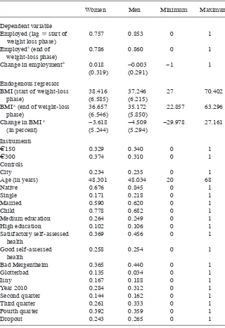
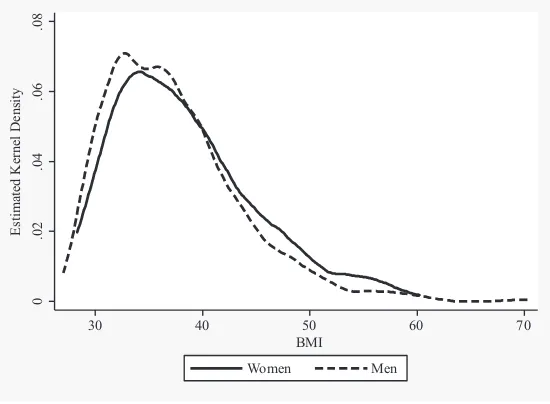
Descriptive statistics at the start of the intervention period are presented in Table 1. Less than one- third (32 percent) of the participants are women. Most participants (76 percent of women and 85 percent of men) were employed before the interven-tion. The average BMI of female participants was 38.4, which was a little higher than the BMI of male participants (37.2). The distribution of the BMI by sex before the weight- loss intervention is displayed in Figure A2 in the appendix.
About 33, 37, 17, and 14 percent of the female participants were recruited by the clinic in Bad Kissingen, Bad Mergentheim, Isny, and Glottertal, respectively. The shares of male participants recruited by the clinic in Bad Mergentheim and Isny are considerably higher. In contrast, the clinic in Glottertal recruited signifi cantly fewer male than female patients. Around 25 percent of the observations fi nished the tenth grade of secondary school. The share of participants with at least a high school degree amounts to 10 percent. All other participants have a lower (or unknown) educational attainment. The average age is about 48 years. Most participants (78 percent) were born in Germany. This group is signifi cantly larger among men. More than 25 percent of the participants reported a good health status.
The randomization algorithm yielded an even distribution across the three groups, which indicates that the randomization procedure worked properly. Table 2 shows that, before the weight- loss intervention, there are no signifi cant group differences with respect to employment or BMI. Also, most covariates are balanced between the ex-perimental groups (Table A2 in the appendix). Chance variability always will produce some differences between experimental groups. A test whether observed group differ-ences in the distribution of the covariates actually are attributable to chance (Hansen and Bowers 2008) warrants exogeneity of group membership.
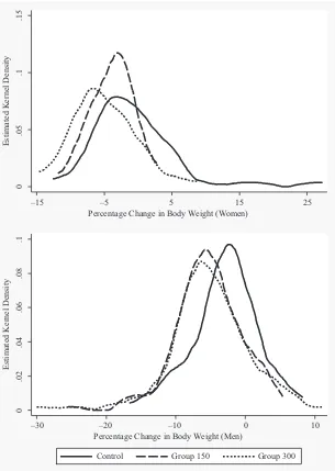
During the intervention period, however, signifi cant differences between the control and the two incentive groups among both female and male participants have arisen (Table 2). With respect to weight loss measured in percent of BMI, female members of the control group lost, on average, 0.6 percent, while women being rewarded with €150 and €300 lost 3.9 and 5.1 percent, respectively. The difference in weight loss between the two premium groups is insignifi cant (p- value of 11 percent). Male mem-bers of the incentive groups also lost more weight than men in the control group. The distribution of weight loss by experimental groups and gender is displayed in Figure A3 in the appendix. Moreover, the shares of participants in employment developed differ-ently across experimental groups (only among women). Whereas the share of employed women declined in the control group, it remained unchanged in the group with the €150 reward and increased in the group with the €300 reward. The difference between the latter group and the control group is statistically signifi cant, indicating improved employment prospects due to the higher reward. Observing (signifi cant) differences between the premium groups and the control group with respect to both weight loss and employment prospects among female participants suggests a causal link between obesity and employment of women. Estimating its magnitude is the aim of the paper.17
Reichert 767
3.618 −4.509 −29.978 27.161
(5.244) (5.294)
Age (in years) 48.301 48.034 20 68
Native 0.676 0.845 0 1
Single 0.171 0.218 0 1
Married 0.590 0.620 0 1
Child 0.778 0.682 0 1
Medium education 0.264 0.249 0 1
High education 0.102 0.106 0 1
Satisfactory self- assessed
Bad Mergentheim 0.365 0.440 0 1
Glotterbad 0.135 0.034 0 1
Isny 0.167 0.188 0 1
Year 2010 0.284 0.312 0 1
Second quarter 0.144 0.162 0 1
Third quarter 0.261 0.333 0 1
Fourth quarter 0.392 0.359 0 1
Dropout 0.243 0.265 0 1
The Journal of Human Resources 768
IV. Estimation Strategy
The purpose of the analysis is to investigate whether there is a causal association between body weight and employment prospects, which is diffi cult be-cause body weight may suffer from endogeneity due to unobserved heterogeneity. For instance, individual time preference may be simultaneously correlated with diffi cul-ties in timing food intake and task completion on the job. In this case, the correlation between body weight and employment prospects may capture the effect of a high discount rate. Moreover, employment may affect weight. A more detailed argumenta-tion of potential sources of bias is provided by Norton and Han (2008).
One way to control for endogeneity and reverse causality is by employing two- stage least squares regression.18 IV estimation solves this problem by using only the part of the variability in weight orthogonal to employment prospects to estimate its pure effect on employment. IV estimation requires variables that are correlated with weight but otherwise unrelated to employment. I use the two premium group indicators as instru-ments. Because the monetary rewards were paid contingent on the change in body weight and the correlation between the instrumental variables and post intervention BMI is rather weak due to sample heterogeneity in baseline body weight, I estimate the econometric model in fi rst differences. The resulting correlation between the in-strumental variables and BMI growth is substantial. As the premium group indicators are furthermore uncorrelated with unobserved factors due to the experimental design, they represent suitable instruments for weight change.
Theoretically, one would not need to include covariates into the econometric model. However, randomization may yield a random imbalance of some covariates in a fi nite sample (Lock 2011). Another source of inconsistency may arise due to sample attrition.19
18. Estimators that attempt to eliminate the fi nite- sample bias of two- stage least squares such as limited information maximum likelihood and jacknife IV estimators (Blomquist and Dahlberg 1999) confi rm two- stage least squares regression results.
19. IV estimation yields consistent parameter estimates if the instrumental variables are correlated with the endogenous regressor and uncorrelated with the error term. Both conditions, especially instrument exogene-ity, may be violated in the presence of sample selection.
Exclusion restrictions for sample selection
Pharmacy in town 0.631 0.638 0 1
Cholesterol test 0.590 0.568 0 1
Blood glucose test 0.851 0.818 0 1
Number of observations 222 468
Notes: Standard deviations for binary variables omitted. No statistics for reference category reported. Means do not include observations with missing values. Bad Mergentheim, Glotterbad, and Isny refer to the loca-tions of the rehabilitation clinics.
a. For participants who attended the control weigh- in only. Number of observations: 168 (Women) and 344 (Men).
Reichert
769
Table 2
Dependent and Main Explanatory Variable by Experimental Groups
Women Men
Women Men Control €150 €300 Control €150 €300
At experiment initiation
BMI 38.416 37.246 38.162 38.309 38.714 36.77 37.318 37.705 (6.585) (6.215) (6.521) (5.918) (7.23) (5.641) (6.600) (6.401) Employed 0.757 0.853++ 0.773 0.795 0.711 0.890 0.824 0.841
Number of observations 222 468 66 73 83 164 159 145 During treatment period
Change in BMI −3.618 −4.509 −0.588 −3.903** −5.109** −2.949 −5.325** −5.183** (In percent) (5.244) (5.294) (6.787) (3.332) (4.742) (4.789) (4.818) (5.870) Change in employment 0.018 −0.003 −0.073 0.000 0.082** –0.027 0.026 −0.008
(0.319) (0.291) (0.346) (0.336) (0.277) (0.285) (0.311) (0.276) Number of observations 168 344 41 54 73 111 114 119
Notes: ++ deviation from women signifi cant at 5 percent, + deviation from women signifi cant at 10 percent; ** deviation from control group signifi cant at 5 percent, **
deviation from control group signifi cant at 10 percent. ^^ deviation from group with €150 reward signifi cant at 5 percent, ^ deviation from group €150 reward signifi cant at
The Journal of Human Resources 770
Table 1 shows that several participants dropped out of the study. If dropping out of the sample is highly correlated with receiving fi nancial incentives for weight loss, IV estimation may yield inconsistent estimates although the direction and magnitude of the bias would not be a priori clear.20
The inclusion of covariates may remove both sources of inconsistency because, on the one hand, it eliminates a possible random correlation with the instruments and a potential random correlation of the instruments with unobserved variables on the por-tion of their associapor-tion with the covariates (Imai, King, and Stuart 2008). On the other hand, the covariates control for potential nonrandom sample attrition under the assump-tion that the decision to drop out from the experiment is entirely determined by the observable factors. This means it is required that, conditional on the covariates, sample attrition is purely random. In Section VI, I test this assumption. A further attractive feature of including the regressors is that they reduce the variance of the employment effect of weight loss, hence, increasing the effi ciency of the estimate (Vance and Ritter 2012). Because baseline values are unaffected by the experiment and most covariates do not change over time, I exclusively use the baseline values for covariates.
Accordingly, I set up a regression model that explains the change in employment,
Ei,t – Ei,t–1, by a percentage change in BMI21, and a vector of control variables, X i,t–1:
E
i,t− Ei,t−1= Xi′,t−1+[(BMIi,t−BMIi,t−1) / BMIi,t−1 ]+εi,t.
Subscript i and t indicate the individual and time, ε represents a random error term, while and are coeffi cient vectors subject to estimation. Instead of the percentage change in BMI, two- stage least squares estimation employs the fi tted values from a regression of the percentage change in BMI on the two instrumental variables and
Xi,t–1. Corrected and heteroscedasticity- robust standard errors are computed.
Note that due to the relatively low number of observations, a limited number of covariates is preferably employed in order to guarantee numerical stability of the es-timation. Covariates with a missing value were assigned the value of 0 (there are no missing items for the BMI) and a binary indicator controlling for the corresponding observations is included. The sex of six participants is imputed based on height and employment information.22 The basic model specifi cation accounts for the
rehabilita-20. Assessing the possible bias implied by naively comparing observed group means of weight- loss success for the same fi nancial incentive scheme, Augurzky et al. (2012) prove that both an upward bias and a downward bias may occur. For the present empirical analysis, this implies that the direction of a possible bias due to sample selec-tion is a priori unclear in the fi rst- stage equation of the IV estimation. The direction of a possible attrition bias in the reduced- form (the numerator of the IV coeffi cient) is similarly diffi cult to predict. For instance, it may be that individuals who lose the job are more likely to continue with the experiment due to time constraints that fall away. On the other hand, they may have lost their daily routine that makes it diffi cult for them to meet the weigh- in deadline and to stay in the experiment, respectively. Hence, the direction of a potential sample- selection bias is a priori unclear for the IV coeffi cient as a whole. To recall the formula of the IV coeffi cient, see Footnote 24. 21. Percentage change in BMI levels weight loss achievement across initial BMI values. Using the change in BMI or weight loss in kilograms yields qualitatively the same results.
Reichert 771
tion clinics, living in a city, time dummy variables indicating the quarter and year of experiment initiation, and basic socioeconomic variables. In my preferred model specifi cation, dummy variables indicating educational attainment and self- assessed health are additionally included.
V. Results
First, I briefl y discuss OLS results as reference. The upper panel of Table 3 displays that only few covariates have a signifi cant effect. Importantly, the percentage change in BMI is insignifi cant for both sexes irrespective of which covari-ate set is considered in the regression. The only signifi cant result among women is that patients treated in the clinic of Bad Mergentheim have better employment pros-pects than patients treated in the clinic of Bad Kissingen (reference category), which points to the type of disease being relevant for labor market prospects. Among men, only the coeffi cient of age is signifi cant, pointing to worse employment prospects of older men.
Concerning the IV estimation results, I fi nd a statistically signifi cant negative effect of percentage change in BMI on employment for women in both model specifi cations. This means that obese women who lose weight improve their em-ployment prospects. For men, in contrast, the negative coeffi cient of weight loss is insignifi cant and considerably smaller.23 Compared to OLS, IV results yield larger coeffi cients for percentage change in BMI in absolute terms. This is an indication that unobserved factors or reversed causation mask the causal effect of weight loss on employment.
Turning to the results for the fi rst- stage equation (lower panel of the tables), I observe signifi cant coeffi cients for age among both women and men, pointing at a lower weight- loss success for older participants. The same pattern is observed for women living in urban areas and men with high educational attainment. Irrespective of the sex considered, the instrumental variables exhibit the expected negative sign and generally confi rm the results of Augurzky et al. (2012). Women who are prom-ised €150 for weight loss reduce their body weight by about 3.7 percentage points (standard error: 1.1) more than the control group. If they are promised €300 for achieving the target weight they even lose 5.1 percentage points (standard error: 1.2) more than the control group. The differential effect of the higher reward is statisti-cally signifi cant. In the regression for men, the coeffi cients of the instrumental vari-ables are also signifi cant and slightly stronger than in the regressions for women. The joint tests on instrument relevance yield F- statistics of 9.0 (women) and 9.5 (men) that are below the critical threshold (for two instrumental variables and one endo-geneous regressor) of 19.93 suggested by Staiger and Stock (1997) and, hence, not very strong. However, since they are orthogonal to employment, they do not incur
772
Table 3
IV Effects on Employment Prospects by Gender
Women Men
OLS IV OLS IV
Covariate Set Basic Extended Basic Extended Basic Extended Basic Extended
Structural equation: change in employment
Change in BMI (in percent) −0.001 −0.002 −0.026** −0.026** −0.005 −0.005 −0.012 −0.010 (0.005) (0.005) (0.013) (0.012) (0.003) (0.003) (0.013) (0.014) Age −0.003 −0.003 −0.001 −0.001 −0.005** −0.005** −0.005** −0.004**
(0.003) (0.003) (0.003) (0.003) (0.002) (0.002) (0.002) (0.002) Native −0.006 0.020 0.011 0.045 −0.039 −0.030 −0.046 −0.036
(0.056) (0.059) (0.059) (0.060) (0.051) (0.050) (0.054) (0.053) Married −0.030 −0.031 −0.034 −0.029 −0.011 −0.011 −0.010 −0.010
(0.056) (0.057) (0.061) (0.059) (0.045) (0.047) (0.045) (0.046) Single −0.036 −0.023 −0.040 −0.015 0.083 0.089 0.088 0.093
(0.105) (0.100) (0.113) (0.102) (0.077) (0.077) (0.075) (0.075) Having kids −0.075 −0.057 −0.097 −0.070 0.099 0.101 0.089 0.093
(0.062) (0.061) (0.076) (0.068) (0.063) (0.062) (0.066) (0.065) City 0.084 0.089 0.116 0.124 0.016 0.022 0.019 0.025
(0.099) (0.096) (0.094) (0.092) (0.035) (0.036) (0.035) (0.035) Bad Mergentheim 0.122* 0.129* 0.142* 0.147** −0.038 −0.040 −0.044 −0.044
(0.070) (0.071) (0.073) (0.072) (0.037) (0.038) (0.038) (0.038) Glotterbad 0.012 0.011 0.027 0.029 −0.031 −0.022 −0.033 −0.024
773
Isny 0.009 0.019 −0.019 −0.006 −0.037 −0.033 −0.045 −0.039 (0.063) (0.068) (0.054) (0.057) (0.041) (0.041) (0.043) (0.043)
Medium education −0.024 −0.033 0.035 0.037
(0.062) (0.065) (0.038) (0.037)
High education 0.083 0.136 −0.021 −0.012
(0.078) (0.088) (0.053) (0.057) Satisfactory self- assessed health −0.021 −0.003 −0.003 −0.006
(0.060) (0.060) (0.047) (0.047) Good self- assessed health −0.016 0.005 −0.015 −0.018
(0.059) (0.057) (0.044) (0.042) Constant 0.180 0.137 0.010 −0.068 0.187 0.141 0.144 0.110
(0.178) (0.197) (0.233) (0.252) (0.147) (0.153) (0.172) (0.177) First- stage equation:
change in BMI (in percent)
€150 −3.834** −3.652** −2.489** −2.521**
(1.155) (1.126) (0.634) (0.618)
€300 −5.002** −5.134** −2.412** −2.359**
(1.234) (1.208) (0.715) (0.721)
Age 0.077* 0.079* 0.062* 0.056*
(0.044) (0.041) (0.032) (0.033)
Native 0.971 1.306 −1.081 −0.998
(0.997) (0.867) (0.846) (0.827)
Married 0.055 0.236 −0.005 0.077
(0.939) (0.952) (0.765) (0.799)
Single 0.229 0.543 0.735 0.715
(1.704) (1.554) (1.075) (1.097)
Having kids −0.815 −0.588 −1.279 −1.308
(1.435) (1.335) (0.891) (0.909)
774
Women Men
OLS IV OLS IV
Covariate Set Basic Extended Basic Extended Basic Extended Basic Extended
City 1.756* 1.948** 0.644 0.600
(0.932) (0.898) (0.835) (0.826)
Bad Mergentheim 0.857 0.958 −1.018 −0.897
(1.023) (0.990) (0.641) (0.625)
Glotterbad 0.071 0.259 −0.555 −0.512
(1.336) (1.221) (1.174) (1.104)
Isny −1.412 −1.326 −1.147 −1.065
(0.943) (0.985) (0.799) (0.767)
Medium education −0.280 0.410
(0.826) (0.661)
High education 2.195 1.773*
(1.409) (0.918)
Satisfactory self- assessed health
0.765 −0.709
(0.942) (0.641)
Good self- assessed health 0.189 −0.630
(0.978) (0.809)
Constant −4.455 −6.002* −4.521* −4.085
(3.382) (3.086) (2.441) (2.569) Number of observations 168 344
Notes: ** signifi cant at 5 percent, * signifi cant at 10 percent. Robust standard errors in parentheses. Missing values of covariates set to zero. ”Missing” indicator included. Results for dummy variables indicating the year and the quarter not reported. Bad Mergentheim, Glotterbad, and Isny refer to the locations of the rehabilitation clinics.
Reichert 775
a meaningful bias.24 Weak- instrument robust tests (Finlay and Magnusson 2009) confi rm the fi nding of weight loss signifi cantly improving employment prospects of women and no effects for obese men. This fi nding is further warranted by using a joint treatment- group indicator (grouping treatment- group members irrespective of being promised €150 or €300 for weight loss) as a single instrument for weight loss, which turns out to be suffi ciently strong (F- statistics above 16) in the IV re-gressions (Table A6 in the appendix).
Regressing the outcome variable directly on the instruments for weight loss (but not weight loss itself, then estimating the reduced form) including the same regres-sors, yields signifi cant effects on employment prospects for women, too. The test of joint signifi cance of the two group indicators reveals that fi nancial rewards contingent on (partially) achieving a weight- loss target of between 6 and 8 percent within four months signifi cantly improve the employment prospect of obese women. The coef-fi cients of the two rewards do not signifi cantly differ (p- value of 17.4 percent). Finan-cially rewarding obese men, in contrast, is not a promising policy option. The results are presented in Columns 1 and 2 of Table A1 in the appendix.
VI. Sample Selection
In order to test the hypothesis of no selection problem (because of the dropouts) in the presence of an endogenous explanatory variable, I follow the test sug-gested by Wooldridge (2010), which is based on the inverse Mills ratio in a Heckman (1976, 1979) selection model.25 Sample selection is then a problem if the t- statistic for the coeffi cient of the inverse Mills ratio is signifi cant in an IV regression.
The design of the experiment renders several variables well suited as exclusion re-strictions. In particular, I use variables not associated with weight reduction that relate to the distance from the assigned pharmacy (“pharmacy in town”) and the availabil-ity of cholesterol as well as blood glucose tests in the pharmacy.26 Being assigned a nearby pharmacy is assumed to be positively correlated with program continuation because time and transportation costs are low. The availability of the respective blood tests may be negatively associated with sample attrition due to gains of being informed
24. This is nicely illustrated by the IV formula ˆIV
=(Z Y′ /Z X′ )=+(Z′ε/Z X′ ), where y is the depen-dent variable, Z the instrumental variable, ε the error term, and X the vector of covariates; see also Murray (2006). Note that the instrumental variables pass the overidentifi cation tests. P- values on the test of overiden-tifying restrictions range between 0.38 (basic covariate set) and 0.54 (extended covariate set) for women as well as 0.45 and 0.40 for men. That said, overidentifi cation tests provide limited evidence for instrument validity because both instrumental variables presumably operate on employment through the same channel. 25. Wooldridge (2010) suggests running a probit regression of the selection indicator on the instruments of the endogenous explanatory variables, the exogenous explanatory variables, and at least one variable that affects selection but is otherwise uncorrelated with the outcome variable using all observations. Then, the estimated inverse Mills ratio is obtained. As a second step, he proposes to carry out an IV regression of the outcome variable on the exogenous and instrumented endogenous explanatory variables including the esti-mated inverse Mills ratio as an additional regressor. For the second step, the selected subsample (individuals that did not drop out) is used.
The Journal of Human Resources 776
although participants may likewise consider participation in the blood tests as wasting time or fear the prick that is involved with the blood test.
The probit results for the selection equation, where I use a dummy variable for drop-ping out of the sample as the dependent variable, are presented in Columns 3 and 6 of Table A7 (women) and Table A8 (men) in the appendix. As expected, being assigned a pharmacy in town signifi cantly reduces the dropout likelihood of women and men. With respect to the blood tests, the availability of a cholesterol test and a blood sugar test is a signifi cant correlate of study continuation for women and men, respectively. For brevity, I do not discuss full IV regression results but mention only the results for the test on the coeffi cient on the estimated inverse Mills ratio. I fi nd no evidence of a selection bias due to sample attrition among women. In particular, the p- value of the coeffi cient of the inverse Mills ratio for women is 0.80 (basic covariate set) and 0.73 (extended covariate set). Moreover, the estimated weight- loss effects remain virtually the same across the specifi cations. For men, the test statistics do not indicate a sample selection problem either.
Further sample selection checks presented in the appendix focus on the estimation of worst- case reduced- form- effect bounds and show the robustness of the results with respect to accounting for sample selection. This is evidence for sample attrition be-ing of minor relevance for the numerator of the IV coeffi cient. Because extensive empirical examinations of Augurzky et al. (2012) point at sample attrition being also of minor relevance for the denominator of the IV coeffi cient, sample- selection bias represents a minor concern for the IV coeffi cient as a whole. This is in line with my theoretical consideration regarding the magnitude of the bias in Section IV and war-rants sample- selection- test results reported above.
VII. Effect Size and Employment Legislation
Having established a statistically signifi cant effect that is robust to sample attrition, two questions remain: fi rst, whether the effect is of economic rel-evance and, second, whether fi nding any effect is plausible given the relatively short intervention period.
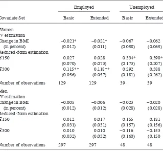
For a discussion of the effect size, I estimate separate regressions for participants that were employed and participants that were unemployed at the start of the experiment. This is necessary because the above presented coeffi cients capture the effect of the change in body weight on the change in employment, which is diffi cult to interpret. In contrast, interpretation of separate IV regression estimates for the two initial employ-ment states is straightforward. For previously employed participants, they yield the effect of weight loss on the probability of remaining employed. For the previously un-employed, they yield the effect on the job- fi nding probability. Likewise, reduced- form estimates yield the respective effects of the monetary rewards. Results are presented in Table 4. More comprehensive results are presented in Tables A9 (women) and A10 (men) in the appendix.
Reichert 777
of 75.7 percent. The estimated reduced- form effects indicate that only the higher mon-etary reward signifi cantly increased the employment probability among previously em-ployed obese women. The coeffi cient is signifi cantly higher than the coeffi cient of the lower reward. Hence, while the reward of €150 does not exert any signifi cant effect, promising obese women that are currently employed €300 for moderate weight loss increases their probability of remaining employed by 11.8 percentage points (standard error: 5.7). This is an effect of economically meaningful size.
The estimated effect on the job- fi nding probability of obese women who were unemployed at the start of the experiment—though insignifi cant—tends to be even larger. Particularly large coeffi cients are found in the reduced- form estimation. The effect of the reward of €150 is even statistically signifi cant (p- value of 5.9 percent) whereas the differential effect of the higher reward is not. However, due to the very small sample size, these estimates have to be interpreted with caution. In light of the estimates based on the joint female sample, I would therefore consider −2.1 percentage Table 4
Effects on Employment Prospects by Initial Employment Status
Employed Unemployed
Covariate Set Basic Extended Basic Extended
Women IV estimation Change in BMI
(in percent) −
0.021* −0.021* −0.067 −0.062
(0.012) (0.011) (0.058) (0.065)
Reduced- form estimation
€150 0.027 0.028 0.334* 0.390*
(0.070) (0.073) (0.173) (0.207)
€300 0.115** 0.118** 0.292 0.388
(0.056) (0.057) (0.181) (0.262)
Number of observations 129 129 39 39
Men
IV estimation Change in BMI
(in percent) −
0.005 −0.006 −0.023 −0.020
(0.012) (0.012) (0.028) (0.028)
Reduced- form estimation
€150 0.012 0.017 0.155 0.181
(0.031) (0.031) (0.157) (0.156)
€300 0.010 0.010 −0.116 −0.153
(0.032) (0.032) (0.160) (0.150
Number of observations 297 297 48 48
The Journal of Human Resources 778
points to be an appropriate conservative estimate for the effect of a percentage change in BMI on the job- fi nding probability of previously unemployed obese women. Re-garding the effects for obese men, I neither fi nd signifi cant effects on the probability of remaining employed of the previously employed nor on the job fi nding probability of the previously unemployed.27
An absolute estimate of roughly two percentage points for the effect on the prob-ability of employment seems to be economically relevant but more must be said about the plausibility of fi nding any signifi cant employment effects in the light of the rela-tively short intervention period and German employment legislation. In order to do so, I aim to corroborate both observed transitions out of employment of participants who were employed and transitions into employment of participants who were unemployed at the start of the experiment.
Dismissal regulation is relevant for transitions out of employment.28 A legal re-quirement for dismissals is that the notice period is respected. Being consecutively employed by the same employer for two, fi ve, eight, and ten years implies a notice period of one, two, three, and four months, respectively. For continuous employment of more than ten years, the notice period exceeds four months. Companies with fewer than 20 employees are allowed to offer work contracts with a notice period of one month (Seifert and Funken- Hotzel 2004).
However, any notice period may be consistent with observed transitions out of em-ployment if participants were given the notice prior to the start of the experiment. In this case, the layoff likelihood is necessarily uncorrelated with weight change during the intervention period, which, at fi rst glance, contradicts my fi nding of weight loss positively affecting the probability of remaining employed. However, transitions out of employment need to satisfy two conditions: the loss of the current job and lack of success in fi nding a new job. This implies that observed effects on the probability of remaining employed can plausibly be explained based on effects on the probability of fi nding a new job alone. Consistent with this argument, I observe that about as many participants changed employer during the intervention period as participants lost their job.29 Therefore, the plausibility of the four- month horizon for the effects on the job- fi nding probability (see discussion below) becomes more relevant.
In light of the legal requirements discussed, the observed transitions out of employ-ment are also possible if participants were actually given notice during the
interven-27. Following the two- step estimation procedure of Rivers and Vuong (1988), results for the effects on the probabilities of remaining employed and fi nding a job are qualitatively the same as those from the linear model (yet, in absolute terms, the nonlinear model yields slightly lower point estimates).
28. In Germany, dismissals must be justifi ed on grounds related to the employee’s person, her behavior, or the economic situation of the company. Dismissals for reasons concerning the employee’s personality require that employees are not (or no longer) able to fulfi ll their tasks. Health- related dismissals are explicitly included and are, in practice, the most common form within this dismissal category. A general rule of thumb is that more than six weeks of sickness absence within 12 months justifi es a dismissal (FOCUS- Online 2013). This criterion is fulfi lled by all participants who made transitions out of employment. On average, they were 58 days absent from work in the course of four months prior to medical rehabilitation participation. Dismissals for reasons concerning the employee’s behavior are violations of obligations resulting from the employment contract. Dismissals for economic reasons can be internal, such as organizational restructuring, or external to the employer. Here, the employer is obliged to select employees with the shortest length of service, lowest age, fewest dependent family members and lowest degree of disability in the case of several dismissal candidates.
Reichert 779
tion period rather than prior to the start of the experiment. Among participants who made a transition out of employment, about 27 percent were at least once unemployed in the last three years before the start of the experiment. Their notice period was less than four months. For all other participants, I do not know their notice period. How-ever, relevant statistics for Germany indicate that less than four months is indeed a plausible estimate for their notice period. For instance, Hobijn and Sahin (2009) show that the average share of German employees with more than ten years of tenure usu-ally amounts to only 40 percent. Moreover, a notice period of one month applies to a substantial fraction of German employees who work for companies with fewer than 20 employees.30
Four months are also suffi cient for observed transitions into employment. Hobijn and Sahin (2009), for instance, report that usually about 7 and 18 percent of the Ger-man unemployed fi nd a job within one month and three months, respectively. This is confi rmed by German employer survey data, which reveal that the average recruitment period between publishing a vacancy and starting the job amounts to 77 days (Brenzel et al. 2008). This fi gure is even lower in the low- pay sector (only about 40 days) as many potential workers match the required skills (van Ours and Ridder 1992; Heck-mann, Noll, and Rebien 2013). Hence, since the majority of participants and virtually all participants who are unemployed at the start of the experiment are low- skilled, observed effects on the job fi nding probability are well in line with the intervention period.
VIII. Potential Mediators of Weight Loss
In this section, I discuss whether the fi nancially induced weight loss is large enough to operate through potential mediators on employment. Moreover, I aim to provide further support for the positive effect of weight loss on the employment prospects of obese women by looking at the effect of weight loss on two potential mediators for employment.
While a variety of potential mediators of weight loss are already discussed above (Section II), I subsequently address the question whether they are plausibly activated by an induced weight loss of about 5 percent (as observed for women of the €300 reward group, displayed in the lower panel of Table 3). In doing so, I, for example, refer to considerable improvements in health and health- related quality of life that were shown to result from weight loss of about only 5 percent in obese people (Bilger et al. 2013, Villareal et al. 2011, Imayama et al. 2011).31 That health is an important determinant of employment outcomes is well documented in the relevant literature (for example, García- Gomez et al. 2013).
Plausibility is further warranted by the fact that a 5 percent weight loss represents a conservative estimate for the reduction in body fat mass. Villareal et al. (2011), for instance, show in a randomized trial of diet and exercise interventions that effects are, in absolute terms, about 1.7 times higher on fat mass than on body weight. As opposed
30. In Germany, the share of employees working for fi rms with fewer than 20 employees historically exceeds 20 percent (Bauer, Schmucker, and Vorell 2008).
The Journal of Human Resources 780
to fat- free mass, only fat mass was shown to be of relevance for the probability of em-ployment among women (Burkhauser and Cawley 2008, Johansson et al. 2009). This is explained by adverse health effects of obesity being entirely attributable to body fat provided that fat- free mass is rather positively associated with physical fi tness (Bigaard et al. 2004). Moreover, discrimination is arguably only related to fat mass.
Next, I probe whether effects of weight loss on potential mediators actually can be seen in the data. Although proxy variables for most mediators are lacking, I have two suitable measures of labor productivity. I argue that fi nding positive effects of weight loss on proxy variables for labor productivity for women (but not for men) lends credence to the fi ndings in Section V.
One variable relates to physical well- being and the other to limitations at daily tasks due to health complaints. Physical well- being is thought of as a proxy variable for self- esteem and self- confi dence, which are considered as contributors to working productivity32, and is in an ordinal scale, taking on values from one (very good) to fi ve (bad). Limitations at daily tasks due to health complaints indicate how well individu-als may be used for physical work or more generally as a proxy for the health status. The participants were asked whether any of the following limitations applies: walking quickly or a long distance, lifting heavy objects, bending, kneeling, and stooping. The respondents could also tick that none of the limitations applies. Descriptive statistics of these variables at experiment initiation are displayed in Table A11 in the appendix.
In order to eliminate random group differentials in the dependent variables at the start of the experiment, the change in the two variables rather than the post- treatment levels enter linear IV regressions as dependent variables. The estimation results are presented in Table 5. For women, the effect of a change in BMI (in percent) on self- assessed physical well- being is negative and signifi cant (p- value of 7.1 percent). This is evidence for weight loss improving self- confi dence of obese women. A signifi cant positive effect is found for the change in BMI on limitations at daily tasks due to health complaints (p- value of 5.3 percent). This means that weight loss also improves physical fi tness of women.33 For men, signifi cant effects are found neither on physi-cal well- being nor on the limitations at daily tasks. Thus, the effect on both proxy variables for labor productivity supports the idea that weight loss induces labor pro-ductivity gains among obese women, while for men this seems not to be the case. The absence of productivity gains of losing weight for male participants is in line with the results of no effects on their probability to be in employment.
At the same time, observed gender heterogeneity in the response of the two variables to weight loss may explain differences in the employment effects between both sexes. This holds especially for self- assessed physical well- being, as the coeffi cients of weight change in respective regressions are statistically different across both sexes and body- related self- perception is a characteristic that evidently translates into better employment prospects (Mobius and Rosenblat 2006). There are many further potential mediators of weight loss
Reichert 781
and probably all of them are—to some extent—activated differently in women and men. Probably the most obvious mediator that exhibits pronounced gender heterogeneity in re-acting to weight loss is weight discrimination because women experience relatively more weight discrimination. In an experimental study, Giel et al. (2012) fi nd that 42 percent of German human resource professionals would absolutely not hire an obese woman whereas (only) 19 percent would not employ an obese man. Importantly, several studies show that weight loss actually improves attitudes toward (formerly) obese (for example, Fardouly and Vartanian 2012; Latner, Ebneter, and O’Brien 2012; Granberg 2011). Unfortunately, there are no suitable proxy variables for weight discrimination in the data set.
IX. Discussion and Concluding Remarks
This study presents credible estimates for the causal effect of BMI growth on employment. By exploring a unique exogenous source of weight loss, the analysis improves upon the existing empirical literature on this topic. In a randomized controlled experiment, obese rehabilitation patients were successfully motivated to lose weight by monetary rewards of €150 and €300, respectively. This produced valid instrumental variables because random assignment assured that the monetary rewards exclusively operated on the probability to be in employment through the BMI.
I fi nd convincing evidence for weight loss positively affecting the employment prospects of obese women but not of obese men. This result is robust across different Table 5
IV- Effects on Proxy Variables for Labor Productivity
Women Men self- assessed physical well- being
Change in BMI (in percent) −0.066
(0.038) −
Number of observations 158 158 337 337
Fewer limitations at daily tasks
Change in BMI (in percent) −0.031**
(0.016) −
The Journal of Human Resources 782
model specifi cations and with respect to accounting for sample attrition. Considering obese women who were employed at experiment initiation alone, a one percentage point reduction in the BMI within four months increases the probability of remaining employed by 2.1 percentage points compared to a baseline of 75.7 percent. The effect on the job- fi nding probability of obese unemployed women tends to be even larger; however, due to the small number of respective observations, it has to be interpreted with caution.
The parameter estimates do not necessarily apply to all obese women but rather only to those who can be motivated to lose weight by monetary rewards. Because the study population consists of medical rehabilitation patients with symptoms attribut-able to obesity and given the importance of physical health for labor productivity, results should furthermore be best applicable to morbidly obese people.
I fi nd positive effects of weight loss on proxy variables for labor productivity for women but not for men, which lends credence to my fi ndings. While a comprehensive analysis of the heterogeneity in the effects across gender is beyond the scope of the paper, different effects of weight loss on labor productivity may serve as one explana-tion. Nevertheless, there are many further potential mediators of weight loss, which may be affected differently in women and men. Probably the most obvious mediator that exhibits pronounced gender heterogeneity in reacting to weight loss is weight discrimination.
The results fi t well with previous fi ndings for Germany. Caliendo and Lee (2013) report an employment probability differential between obese and healthy weight un-employed German women who are currently searching for a job of fi fteen percentage points. For obese unemployed German men, they fi nd no effect on employment pros-pects. Analysis for other countries yield even stronger estimated effects. For instance, Morris (2007) reports that obese women in the United Kingdom are 23 percentage points less likely to be in employment than nonobese women. Contrary to my results, he fi nds a signifi cant negative effect for obese men that, nevertheless, is lower than the respective effect for obese women. Lindeboom, Lundborg, and van der Klaauw (2010), in contrast, do not fi nd any evidence of labor market effects of obesity for the United Kingdom. For the United States, several research articles fi nd no signifi cant link between obesity and employment, irrespective of gender. These studies do not necessarily confl ict with the results presented here. The divergence may be explained by the employed instruments estimating treatment effects for different compliant sub-populations. It may likewise refl ect that the employment effects of obesity vary across labor market regulations.
Reichert 783
A rough estimate (please see the appendix) of the fi scal effects of the intervention in the absence of general equilibrium effects yields that the reward of €300 has already a benefi t- to- cost ratio larger than one after 40 and 46 days of effect persistence depend-ing on the underlydepend-ing scenario. This means that the reward is already amortized by its fi scal effects alone if the employment effects persist over slightly less than one and a half months. Because the effects of the reward of €150 are mostly insignifi cant, it is outperformed by the reward of €300. Assuming that the employment effects persist over one year, fi nancially rewarding an obese woman for achieving a weight- loss target by €300 causes average expected fi scal net savings of between €2,106 ($2,639 in PPP) and €2,417 ($3,028 in PPP).
Appendix A
Worst- Case Reduced- Form Effect Bounds
For the estimation of worst case reduced- form- effect bounds, I fol-low two different approaches that are both employed and described in more detail in Augurzky et al. (2012).
First, I carry out an “intention- to- treat” analysis by regressing the employment indicator on the exogenous explanatory variables and the two IVs aiming to use all observations irrespective of whether they drop out of the experiment. Because there is no information about employment after the weight- loss period for dropouts, missing data have to be imputed. There exists no consensus on one particular imputation algo-rithm (Hollis and Campbell 1999). Therefore, I follow the most common procedure that assumes that the outcome variable takes on previous values (the values before the weight- loss phase). By doing so, it is implicitly assumed that the outcome remains unaffected (John et al. 2011), implying a zero reduced- form effect for dropouts. In technical terms, this approach substantially adjusts the raw group differential toward zero. The analysis yields reduced- form effects for women that are very similar— though slightly smaller—to those obtained for the selected subsample in terms of size and signifi cance. This is displayed in the fi rst four columns of Table A1. Regarding men, the intention- to- treat results confi rm the absence of effects. Thus, for both sexes the intention- to- treat analysis substantiates previous sample selection test results.