JIGSAW: THE ISIS3 BUNDLE ADJUSTMENT FOR EXTRATERRESTRIAL
PHOTOGRAMMETRY
K. L. Edmundson*, D. A. Cook, O. H. Thomas, B. A. Archinal, R. L. Kirk
Astrogeology Science Center, U.S. Geological Survey, Flagstaff, AZ, USA, 86001 - [email protected]
Commission IV, WG IV/7
KEY WORDS: Bundle Adjustment, Estimation, Extraterrestrial, Planetary, Space
ABSTRACT:
The Integrated Software for Imagers and Spectrometers (ISIS) package was developed by the Astrogeology Science Center of the U.S. Geological Survey in the late 1980s for the cartographic and scientific processing of planetary image data. Initial support was implemented for the Galileo NIMS instrument. Constantly evolving, ISIS has since added support for numerous missions, including most recently the Lunar Reconnaissance Orbiter, MESSENGER, and Dawn missions, plus support for the Metric Cameras flown onboard Apollo 15, 16, and 17. To address the challenges posed by extraterrestrial photogrammetry, the ISIS3 bundle adjustment module, jigsaw, is evolving as well. Here, we report on the current state of jigsaw including improvements such as the implementation of sparse matrix methods, parameter weighting, error propagation, and automated robust outlier detection. Details from the recent processing of Apollo Metric Camera images and from recent missions such as LRO and MESSENGER are given. Finally, we outline future plans for jigsaw, including the implementation of sequential estimation; free network adjustment; augmentation of the functional model of the bundle adjustment to solve for camera interior orientation parameters and target body parameters of shape, spin axis position, and spin rate; the modeling of jitter in line scan sensors; and the combined adjustment of images from a variety of platforms.
* Corresponding author.
1. INTRODUCTION
The Integrated Software for Imagers and Spectrometers (ISIS) package (http://isis.astrogeology.usgs.gov/) was developed by the Astrogeology Science Center (ASC) of the U.S. Geological Survey (USGS) in the late 1980s for the cartographic and scientific processing of planetary image data (Gaddis et al., 1997; Anderson et al., 2004). Initially supporting the Galileo NIMS instrument, ISIS has since added support for numerous missions including the Viking orbiters; Mariner 9/10; Clementine; Voyager I/II; Galileo SSI; Pathfinder IMP; Mars Global Surveyor MOC, TES, and MOLA; 2001 Mars Odyssey THEMIS; Lunar Orbiter; Cassini ISS, VIMS, and RADAR; Mars Express HRSC; Mars Exploration Rover (MER) Pancam, Navcam, and Micro-Imager; and Mars Reconnaissance Orbiter (MRO) HiRISE and CTX. ISIS was originally developed in FORTRAN for the VAX/VMS operating system, requiring hardware display buffers for interactive graphics. Programming of ISIS2, beginning in 1992, was primarily in C and FORTRAN using the X-Window Application Programming Interface for the UNIX operating system. This was modernized with the move in late 2001 to ISIS3, using C++ as the primary programming language. Though ISIS2 is still used to support some missions and datasets, the work discussed in this paper relates specifically to ISIS3. Support has been recently added for the Lunar Reconnaissance Orbiter (LRO), MESSENGER, and Dawn missions, and for the Metric Cameras flown onboard Apollo 15, 16, and 17.
The digital image mosaic and digital terrain model (DTM) are two key cartographic products generated from planetary image data. Errors in spacecraft navigation and attitude data lead to misregistration between images in the mosaic and to errors in
the DTM. To minimize these errors, images are controlled using the least-squares bundle adjustment, well known as a key element in the photogrammetric workflow (Brown, 1958). Given a set of two-dimensional point feature measurements from multiple images, this process, in its most general form, simultaneously solves for parameters of image position and orientation in addition to triangulated ground point coordinates. The ISIS3 bundle adjustment module, jigsaw, has undergone recent significant development and continues to evolve to meet the challenges posed by extraterrestrial photogrammetry. In the following, we begin with a discussion of some of these challenges and then report on the current state of jigsaw. Examples from the ongoing processing of Apollo Metric Camera images and images from recent missions such as LRO and MESSENGER are given. Finally we close with a summary of future plans for jigsaw.
2. CHALLENGES IN EXTRATERRESTRIAL PHOTOGRAMMETRY
Extraterrestrial photogrammetry is often characterized in terms of the challenges it presents. Kirk, Howington-Kraus, and Rosiek (2000) divide these into three primary categories; multiplicity of datasets, novel sensors, and unusual geometric and coverage properties.
Planetary imaging systems are typically developed for a single mission, and historically have not been designed for the purpose of rigorous geodetic mapping (notable exceptions being the Metric Camera system flown onboard Apollo missions 15-17 and the High Resolution Stereo Camera (HRSC) on the Mars Express spacecraft). Processing combinations of images
acquired from a variety of sensors separated by long time periods is often required. Beyond the relatively simple frame camera, these include line scan, push frame, and radar sensors for which the time variation of orientation parameters must be modeled. For line scan and push frame sensors, the accurate determination of image position and orientation may also be complicated by unmeasured, high frequency spacecraft motions, or jitter. Sensors may be mounted on orbiting spacecraft or at the surface on stationary platforms or roving vehicles. Images scanned from film cameras on missions long past may be processed together with recent digital images. Images may have vastly different characteristics of illumination, resolution, and geometry. The surfaces of extraterrestrial bodies typically lack any geodetic control. For image exterior orientation (EO), it is necessary then to rely heavily upon spacecraft navigation and attitude data which, particularly from older missions, may have a high level of uncertainty.
Specialized, mission-specific software and sensor models can effectively address general tasks such as image ingestion, pre-processing, and radiometric and geometric calibration. The bundle adjustment must however, exhibit a high degree of generality, flexibility, and efficiency. It must integrate various image sensor data, spacecraft navigation and attitude data, and observations from other sources, such as laser altimeters. Further, it must include available a priori information on target body rotation and overall shape and size. The further development of computationally creative approaches to the bundle adjustment remains relevant as today’s planetary missions generate vast amounts of digital image and other data.
3. THE PHOTOGRAMMETRIC PROCESS IN ISIS3
After ingestion into ISIS3, images are typically calibrated radiometrically and may undergo additional processing for noise removal. Rigorous sensor models define the relationship between ground and image and include system and camera calibration parameters. Initial estimates of image EO parameters are from spacecraft navigation and attitude data which is available in ISIS3 in the form of SPICE (Spacecraft, Planet, Instrument, C-matrix (pointing), and Events) kernels consistent with the standards of NASA’s Navigation and Ancillary Information Facility (NAIF) (Acton, 1996). In the past (prior to the mid 1990’s), operators measured tie points between overlapping images manually. This is now accomplished primarily through automated image matching techniques. Operators can still measure tie points manually, if necessary, and manually correct errors occasionally produced by automated methods. Prior to bundle adjustment, initial ground coordinates of tie points are generated by intersection with an available shape model, such as a sphere, ellipsoid, or global, regional, or local DTM.
At the time of writing, the correction of jitter in line scan sensors has not been fully addressed within ISIS. The University of Arizona (UA) has developed a method to correct for jitter in HiRISE images of Mars. This approach utilizes a jitter modeling tool created at UA together with dedicated ISIS tools (Mattson et al., 2009). The HiRISE camera consists of 14 Charge Coupled Devices (CCDs) arranged in a staggered array on a fixed focal plane. The cross-track overlap and along-track time separation of the CCDs are used to collect information on spacecraft motion. Pixel offsets are measured between feature positions in the overlap area of CCD pairs. From these offsets,
jitter is estimated in the x and y directions and interpreted in terms of camera pointing angles. These are combined with existing pointing data to create an improved NAIF camera pointing kernel. For applications such as map projection, bundle adjustment, and stereo analysis, images resampled with the improved kernel are ideally jitter-free. The smooth orientation data can be bundle adjusted as usual to bring the image into agreement with ground control. This technique may also be applicable to LRO narrow-angle camera (NAC) images. It depends crucially on the fact that stereo parallax can be neglected when comparing features seen in multiple detectors during a single observation. To model jitter in line scan cameras with significant stereo convergence between detectors (e.g. HRSC) it will be necessary to solve simultaneously for ground point coordinates and jitter motion.
4. JIGSAW
Jigsaw is currently capable of adjusting image data from frame and line scan cameras and the Chandrayaan-1/LRO Mini-RF radar sensor. Although Magellan SAR and Cassini RADAR images can be processed in ISIS3, they are produced in map-projected form and are handled as maps rather than images. Currently, only Mini-RF radar images can be bundle adjusted (Kirk and Howington-Kraus, 2008).
Using jigsaw, one may solve for camera pointing alone, camera position alone, or pointing and position simultaneously. Three dimensional coordinates (latitude, longitude, and radius) of all ground points are also determined in the adjustment. Through rigorous weighting, parameters may be held fixed, allowed to adjust freely, or constrained with a priori precision information.
The functional model for the bundle adjustment, defining the relationship between image and object space coordinate systems, is the standard collinearity condition or its radar equivalent, in which a pixel corresponds to a known circle in space rather than to a line. This model is modified for time-dependent line scan and radar sensors to allow for changes in EO parameters between neighboring lines (e.g. Ebner, Kornus, and Ohlhof, 1992; Fraser, 2000). In this case, EO parameters are modeled as functions of time. In jigsaw, individual 2nd or higher order polynomials are utilized as interpolation functions for each EO parameter. In the adjustment of line scan images, it is well-known that high correlations typically occur amongst polynomial coefficients, notably between position and attitude parameters. To control these correlations, the selection and weighting of these parameters must be carefully considered (Fraser, 2000). Alternatives to polynomials such as spline functions are being considered for more accurate representation of EO parameters over long scans.
Several notable improvements to jigsaw have recently been implemented. As mentioned above, the rigorous weighting of parameters allows the a priori precision of spacecraft position, attitude data, and ground point coordinates to be included in the adjustment if available. Similarly, the weight of an image point measurement in the bundle adjustment is computed from its associated a priori precision. In ISIS3, a single precision value can be assigned to all image measurements with the option of specifying any individually. In this way, image points of different precision (e.g., manual vs. automated measurement) can be weighted appropriately. Automated outlier rejection of image measurements via robust M-estimation techniques reduces the need for tedious manual residual analysis (Koch,
1999). The variance-covariance matrix from rigorous error propagation yields estimates of uncertainties for the estimated parameters and any correlations between them. Such estimates are critical to the proper comparison of datasets from different instruments and missions.
With the ever-increasing amount of image data produced by planetary imagers, perhaps the most significant developments in jigsaw are those that have improved computational efficiency and reduced memory requirements. This in turn has dramatically increased productivity. Adjustments that may have previously required many hours or even days are completed significantly faster, for some cases in just minutes. These improvements take advantage of the sparse structure of the normal equations matrix common to aerial and satellite-based photogrammetric networks. Prior to describing these sparse matrix methods, we briefly review least-squares estimation in the Gauss-Markov model and the solution to the normal equations.
4.1 Least-squares Estimation in the Gauss-Markov Model
The subsequent development follows closely Uotila (1986). Given an m x 1 vector l of observables and an n x 1 vector x of unknown parameters, the linear (or linearized) functional model relating the two is
Ax
l−ε= (1)
Where
ε
is an m x 1 vector of true errors and A is the m x n design matrix (m ≥n). Generally, A is of full rank. Given that the expectation of the error vector in (1) is zero, the Gauss-Markov model with full rank is:( )
where D is the dispersion operator, ∑lis the positive-definite
covariance matrix of the observations, σ02 is the a priori
variance of unit weight, and P is the observational weight matrix. The residual vector is given by
l Ax l l
v=ˆ− = − (3)
The “cap” symbol ( ˆ ) indicates an estimated value. The least-squares method yields the estimates xˆ and σˆ02 such that the
Euclidean length of the residual vector is minimized. This leads directly to the normal equations:
0
where n and u are the numbers of observation equations and unknown parameters, and n-u is the degrees of freedom.
Letting N=ATPA andc=ATPl, (5) becomes
c N
xˆ= −1 (7)
N is the normal equations matrix. The variance-covariance matrix of the estimated parameters is given by
(
)
2 14.2 Solving the Normal Equations
The basic form of the normal equations organized by parameter type facilitates a significant reduction in size of the matrix to be solved through parameter elimination (Brown, 1958). The standard approach is to eliminate point parameters. Following Brown (1976), the normal equation system can be written as
⎥
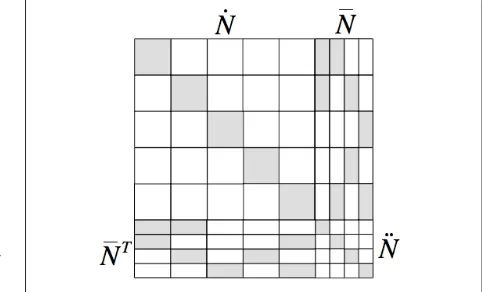
Figure 1 shows the normal equations matrix structure for an example network of five images and four points.N&and c&are contributions to the normal equations with respect to image parameters and N&& and c&&with respect to point parameters. The solution vectors of image and point parameters are x&and&x&. N&
and N&&are block diagonal. N&& consists of 3x3 submatrices
along the diagonal, one for each ground point. N&consists of submatrices on the diagonal for each image, the size of each determined by the number of EO parameters being solved for the image. The elimination of x&& from (9) yields the following reduced normal equation system, the size of which depends only upon the number of image parameters.
(
N&−N N&&−1N T)
x&=c&−N N&&−1&c& (10) The solution vector for the image parameters is x&(
N N N N) (
c NN c)
x&= &− &&−1 T −1 &− &&−1&& (11)
Finally, through back-substitution, the solution vector for the object point parameters is computed from
x
Because N&& is block diagonal, inverting it can be accomplished by the separate inversion of the individual 3x3 submatrices. In practice then, the reduced normal equations matrix is built sequentially by object point, without forming the full N&&or
Figure 1: Structure of full normal equations matrix for an example network with five images and four points. Gray blocks are non-zero, white are zero.
Nmatrices.
In the typical aerial or satellite photogrammetric network the Nmatrix and the reduced normal equations matrix are sparse. In the following section, we discuss how this sparsity may be further exploited.
4.3 Sparse Matrix Methods
Jigsaw uses the CHOLMOD package (Chen et al., 2008; Davis, 2006) for solving the sparse, reduced normal equations. CHOLMOD (for CHOLesky MODification), is a high-performance package for the factorization of sparse, symmetric positive definite matrices and for the modification (update/downdate) of an existing sparse Cholesky factorization. Forming the sparse normal equations matrix efficiently in the bundle adjustment is challenging. The approach adopted here, and the subsequent discussion, follow closely Konolige (2010).
CHOLMOD uses the compressed column storage (CCS) matrix format which is efficient in memory storage but inefficient to fill in an arbitrary manner because the insertion of every non-zero entry requires that all succeeding entries be shifted. To build the reduced normal equations matrix, an interim sparse matrix structure is required that can be efficiently populated in a random fashion and can be traversed by column in row order to subsequently construct the CCS matrix required by CHOLMOD. We use a type of Block Compressed Column Storage (BCCS) which consists of an array of map containers, each representing a column of square matrix blocks in the reduced normal equations (Figure 2). The key into each column map is the block’s row index. The value at each key is a square dense matrix with a dimension equivalent to the number of exterior orientation parameters used for the image. Zero blocks are not stored. The BCCS matrix is created only in the first iteration of the bundle adjustment; in subsequent iterations it need only be repopulated. As the normal equations matrix is symmetric, only the upper triangular portion need be stored.
5. BUNDLE ADJUSTMENT EXAMPLES
In this section we provide examples illustrating the significant time savings resulting from the implementation of sparse matrix methods discussed above. Bundle adjustment results are given for MESSENGER narrow-angle camera (NAC) and wide-angle camera (WAC) images of the planet Mercury, LRO NAC images of the South Pole of the Moon, and a combined network of images from the Metric Cameras flown onboard Apollo missions 15 and 16. We focus here only on the times required per iteration and for the solution of the reduced normal equations. All examples were run on an Intel Xeon X5650 with 16 GB of RAM, 12 MB of cache, and a clock speed of 2.66
GHz. The examples are summarized in Table 1 and details of each follow below.
5.1 Mercury: MESSENGER
The Mercury Dual Imaging System (MDIS) on the MErcury Surface, Space ENvironment, GEochemistry, and Ranging (MESSENGER) spacecraft (Solomon et al., 2001) consists of the monochrome NAC and multispectral WAC frame cameras which are co-aligned and mounted together on a pivot (Hawkins et al., 2007). MDIS acquired images through three flybys of Mercury and has continued to do so since MESSENGER entered orbit around the planet in March 2011 (Solomon et al., 2008). Using these images, the Astrogeology Science Center (ASC) is constructing a global, controlled monochrome base map and DTM of Mercury with ISIS3 (Becker et al., 2012).
The most recent bundle adjustment of MDIS data consisted of 21,498 NAC and WAC G-filter images acquired from a few days after orbit insertion to 15 November, 2011. The network, one of the largest the ASC has processed, contains 263,762 ground points and 1,857,190 image point measurements (3,714,380 observations - two for each measurement). The 855,780 unknown parameters in the adjustment included the coordinates for all ground points (latitude, longitude, and radius) and three attitude angles for all images. The ratio of observations to unknowns is ~4:1. Attitude angles and radius point coordinates were constrained with a priori precisions of 0.2 degrees and 10,000 m respectively. Latitude and longitude point coordinates were free to adjust. The dimension of the reduced normal equations matrix was 64,494. The network exhibits a high degree of sparsity, indicated by the percentage of non-zero entries (0.12%). The total time per iteration was 104 seconds. Of that, 10 seconds were required by CHOLMOD for matrix analysis, factorization, and solution.
Table 1:
Jigsaw
bundle adjustment times for iteration and sparse matrix solution.
Mission
Number of Images
Number of Ground
Points
Number of Image Measurements
Reduced Normals Matrix Dimension
% Sparsity
Time per Iteration (seconds)
Time for CHOLMOD
Analysis, Factorization,
and Solution (seconds)
MESSENGER 21498 263762 1857190 64494 0.12 104 9.95
LRO S. POLE 3827 527756 3363623 22962 3.08 724 121.24
APOLLO 15/16 2664 306457 922573 15984 1.92 65 1.91
Figure 2: Five-image network illustrating the relationship between an upper triangular matrix in dense storage (left) and the same matrix in Block Compressed Column Storage (BCCS) (right). Zero-blocks (in white on the left) are not stored in BCCS format. Numbers inside blocks on the right are row indices.
5.2 The Moon’s South Pole: LRO NAC
With images from the LRO left and right NAC line scan cameras (Robinson et al., 2010), the ASC has produced controlled polar mosaics of the Moon in support of NASA’s Lunar Mapping and Modeling Project (LMMP) (Nall et al., 2010). These are the largest geodetically controlled lunar or planetary mosaics ever produced by the ASC (Lee et al., 2012), and we believe may be the largest such mosaics (in numbers of pixels) ever produced.
The South Pole network contains 3827 images, 527,756 ground points, and 3,363,623 image measurements (6,727,246 observations). The number of unknown parameters was 1,606,230 and the ratio of observations to unknowns ~4:1. While all position and attitude exterior orientation (EO) parameters were modeled by 2nd degree polynomials, only the constant terms for both were included in this adjustment. Position and attitude parameters were constrained with a priori precisions of 1000m and 3.0 degrees respectively. Thirty-seven ground points were constrained in all three coordinates to a Lunar Orbiter Laser Altimeter (Smith, 2010) derived DTM. For the remainder, only the radius coordinate was constrained to the DTM. The dimension of the reduced normal equations matrix is 22,962 and 3% of the matrix entries are non-zero. Time per iteration was 724 seconds and CHOLMOD required 121 seconds for matrix analysis, factorization, and solution. This network contains roughly a sixth of the images in the MESSENGER network, but twice as many ground points and image measurements. A definitive explanation as to why the solution time here seems out of proportion to that of the MESSENGER example and the Apollo Metric example to follow will require more study. It seems likely however that the explanation must in part be related to the relatively higher number of non-zero elements in this matrix.
5.3 The Moon: Apollo Metric Cameras
In the 1970s, an integrated photogrammetric mapping system was among the experiments in the scientific instrument module (SIM) flown on Apollo Missions 15, 16 and 17. This included a frame Metric Camera (MC) for mapping, a high-resolution Panoramic Camera, and a star camera and laser altimeter to provide supporting data. All SIM cameras were film-based. Nearly 25% of the lunar surface was photographed in stereo at resolutions of one to a few meters (Livingston et al., 1980). Later, significant effort was put forth by the Defense Mapping Agency, the National Oceanic and Atmospheric Administration, USGS, and NASA to geodetically control these photographs (Doyle et al., 1976). In 2007, NASA’s Johnson Space Center and Arizona State University (ASU) scanned the original MC negatives at film-grain resolution (Robinson et al., 2008). This work has facilitated an ongoing collaboration between the ASC, the Intelligent Robotics Group of the NASA Ames Research Center (ARC), and ASU, to photogrammetrically and geodetically control that subset of these images with nadir-pointed geometry and in the future, to include oblique images.
The processing of the nadir-pointed imagery has been accomplished with the highly automated Vision Workbench and Ames Stereo Pipeline software (developed by ARC) (Moratto et al., 2010) used in conjunction with ISIS3. Here we report bundle adjustment results for a combined network of Apollo 15 and 16 images. Work on adjusting images from all three missions using jigsaw is ongoing. The Apollo 15/16 network contains 2664 images, 306,457 ground points, and 922,573
image measurements (1,845,146 observations). Both position and attitude EO parameters were included in the adjustment. There are 935,355 unknown parameters and the ratio of observations to unknowns is ~2:1. The dimension of the reduced normal equations matrix is 15,984. 2% of the matrix entries are non-zero. Time per iteration was 65 seconds. Matrix analysis, factorization, and solution were completed in 2 seconds by CHOLMOD.
As a more definitive illustration of the time savings achievable from the application of sparse matrix methods, we cite one further Apollo Metric example for which we have available processing times from a previously implemented dense matrix Cholesky approach. This control network consists of 1462 Apollo 15 images and 168,182 ground points. The time to factorize and solve the reduced normal equations in this case was 31 minutes using the dense Cholesky method. Using CHOLMOD this time was reduced to 0.59 seconds.
6. FUTURE WORK
Here we summarize some capabilities planned for future implementation in jigsaw. Efficient processing of the ever larger data sets generated by planetary missions today requires automating many of the tasks traditionally performed by a human operator. For the bundle adjustment this can be accomplished in part through the implementation of techniques such as robust estimation and sequential estimation. As mentioned in Section 4, robust estimation via M-estimators has recently been implemented in jigsaw. Sequential estimation facilitates the update of an existing data set with new measurements as they become available and the removal of rejected measurements. Free network adjustment (Blaha, 1982) is advantageous for the analysis of measurement residuals free of contamination from errors in constrained parameters. Variance component estimation (Koch, 1986) is important as mixing observations from different sources with unknown precisions is commonplace. We will implement the ability to solve for camera interior orientation parameters and target body parameters of shape, spin axis position, and spin rate. We also intend to pursue the integration and adjustment of data from sensors on multiple platforms including orbiters, descent stages, landers, and rovers. This involves not only multiple coordinate frames but a wide variety of accurately known constraints and less accurately known transformations between them. As mentioned previously, alternatives to general polynomials such as spline functions are being investigated for the representation of EO parameters in images from time-dependent sensors. Finally, based on promising preliminary tests on short images using polynomial fitting, we plan to implement jitter modeling for line scan sensors within the bundle adjustment via spline fitting.
7. ACKNOWLEDGEMENTS
We gratefully acknowledge the MESSENGER mission; the LRO mission, the LROC Science Team, and the Mini-RF Science Team; Mark Robinson from the School of Earth & Space Exploration at Arizona State University; and the NASA Ames Intelligent Robotics Group, in particular Terry Fong, Zachary Moratto, Ara Nefian, and Michael Broxton for their invaluable support and collaboration in the processing of Apollo Metric Camera images. This work has been funded under several NASA programs, including the Planetary
Geology and Geophysics Program, the Lunar Advanced Science and Exploration Research (LASER) program, a grant to Archinal under the LRO Participating Scientist Program, the Lunar Mapping and Modeling Program (LMMP), and the MESSENGER mission.
8. REFERENCES
Acton, C.H., 1996. Ancillary Data Services of NASA’s
Navigation and Ancillary Information Facility. Planetary and Space Science, 44(1), pp. 65-70.
Anderson, J.A. et al., 2004. Modernization of the Integrated Software for Imagers and Spectrometers. Lunar and Planetary Science, XXXV, Abstract 2039.
Becker, K.J. et al., 2012. Global Controlled Mosaic of Mercury
from MESSENGER Orbital Images. Lunar and Planetary Science, XLIII, Abstract 2654.
Blaha, G., 1982. Free Networks Minimum Norm Solution As Obtained by the Inner Adjustment Constraint Method. Bulletin Géodésique, 56(3), pp. 209-219.
Brown, D.C., 1958. A solution to the general problem of multiple station analytical stereotriangulation. RCA Data Reduction Technical Report No. 43.
Brown, D.C., 1976. Evolution and Future of Analytical Photogrammetry. Paper presented to the International Symposium on “The Changing World of Geodetic Science,” Columbus, Ohio 6-8 October, 1976, The Ohio State University.
Chen, Y., Davis, T.A., Hager, W.W., and Rajamanickam, S., 2008. Algorithm 887: CHOLMOD, Supernodal Sparse Cholesky Factorization and Update/Downdate. ACM T Math Software, 35(3), pp. 1-14.
Davis, T.A., 2006. Direct Methods for Sparse Linear Systems. Fundamentals of Algorithms. SIAM, Philadelphia, 217 pages.
Doyle, F.J., Elassal, A.A., and Lucas, J.R., 1976. Experiment S-213 Selenocentric Geodetic Reference System, Final Report, Geodetic Research and Development Laboratory, National Oceanic and Atmospheric Administration, Rockville, MD, and Topographic Division, U. S. Geological Survey, Reston, VA.
Ebner, H., Kornus, W., and Ohlhof, T., 1992. A Simulation Study on Point Determination for The MOMS-02/D2 Space Project Using an Extended Functional Model. In: The International Archives of Photogrammetry and Remote Sensing, Vol. XXIX, Part B4, Amsterdam, pp. 458-464.
Fraser, C.S., 2000. High-Resolution Satellite Imagery: A Review of Metric Aspects. In: The International Archives of Photogrammetry and Remote Sensing, Vol. XXXIII, Part B7, Amsterdam, pp. 452-459.
Gaddis, L. et al., 1997. An Overview of the Integrated Software for Imagers and Spectrometers (ISIS). Lunar and Planetary Science, XXVIII, Abstract 1226.
Hawkins, S. E. III et al., 2007. The Mercury Dual Imaging
System on the MESSENGER Spacecraft. Space Sci. Rev., 131, pp. 247–338.
Kirk, R. L., Howington-Kraus, E., and Rosiek, M.R, 2000. Recent Topographic Mapping at the USGS, Flagstaff: Moon, Mars, Venus, and Beyond. In: The International Archives of Photogrammetry and Remote Sensing, Vol. XXXIII, Part B4, Washington, D.C., pp. 476-490.
Kirk, R. L. and Howington-Kraus, E., 2008. Radargrammetry on Three Planets. In: The International Archives of Photogrammetry, Remote Sensing, and Spatial Information Sciences, Vol. XXXVII, Part B4, Beijing, pp. 973-980.
Koch, K.R., 1986. Maximum Likelihood Estimate of Variance Components, Ideas by A.J. Pope (In memory of Allen J. Pope 11.10.1939-29.08.1985). Bulletin Géodésique, 60(4), pp. 329-338.
Koch, K.R., 1999. Parameter Estimation and Hypothesis Testing in Linear Models, 2nd edition, Springer, Berlin-Heidelberg-New York, 333 pages.
Konolige, K., 2010. Sparse Sparse Bundle Adjustment. In: Proceedings of the British Machine Vision Conference, Aberystwyth, Wales, pp. 102.1-102.11.
Lee, E.M. et al., 2012. Polar Mosaics of the Moon for LMMP.
Lunar and Planetary Science, XLIII, Abstract 2507.
Livingston, R.G. et al., 1980. Aerial Cameras, In Manual of Photogrammetry, 4th Edition, C.C. Slama, C. Theurer, and S.W. Henriksen, Editors. American Society of Photogrammetry, Falls Church, VA, pp. 187–278.
Mattson, S. et al., 2009. HIJACK: Correcting spacecraft jitter in HiRISE images of MARS, European Planetary Science Congress, V4, Abstract EPCS2009-604-1.
Moratto, Z.M. et al., 2010. Ames Stereo Pipeline, NASA’s Open Source Automated Stereogrammetry Software, Lunar and Planetary Science, XLI, Abstract 2364.
Nall, M. et al., 2010. The Lunar Mapping and Modeling
Project. Lunar Exploration Analysis Group Annual Meeting, Abstract 3024.
Robinson, M.S. et al., 2008. The Apollo Digital Image Archive.
Lunar and Planetary Science, XXXIX, Abstract 1515.
Robinson, M. S. et al., 2010. Lunar Reconnaissance Orbiter
Camera (LROC) Instrument Overview. Space Sci. Rev., 150, pp. 81–124.
Smith, D.E. et al., 2010. The Lunar Orbiter Laser Altimeter Investigation on the Lunar Reconnaissance Orbiter Mission.
Space Sci. Rev. 150, pp. 209–241.
Solomon, S. C. et al., 2001. The MESSENGER mission to
Mercury: scientific objectives and implementation. Planet. Space Sci., 49, pp. 1445–1465.
Solomon, S. C. et al., 2008. Return to Mercury: a global
perspective on MESSENGER’s first Mercury flyby. Science, 321, pp. 59–62.
Uotila, U. A., 1986. Notes on Adjustment Computations Part I, Columbus, Ohio: Department of Geodetic Science and Surveying, The Ohio State University.