Using Support Vector Machine for Prediction Dynamic Voltage Collapse in an Actual Power System.

Using Support Vector Machine for Prediction

Dynamic Voltage Collapse in an Actual Power

System

Muhammad Nizam, Azah Mohamed, Majid Al-Dabbagh, and Aini Hussain

Abstract—This paper presents dynamic voltage collapse prediction on an actual power system using support vector machines. Dynamic voltage collapse prediction is first determined based on the PTSI calculated from information in dynamic simulation output. Simulations were carried out on a practical 87 bus test system by considering load increase as the contingency. The data collected from the time domain simulation is then used as input to the SVM in which support vector regression is used as a predictor to determine the dynamic voltage collapse indices of the power system. To reduce training time and improve accuracy of the SVM, the Kernel function type and Kernel parameter are considered. To verify the effectiveness of the proposed SVM method, its performance is compared with the multi layer perceptron neural network (MLPNN). Studies show that the SVM gives faster and more accurate results for dynamic voltage collapse prediction compared with the MLPNN.

Keywords—Dynamic voltage collapse, prediction, artificial neural network, support vector machines.

I. INTRODUCTION

N recent years, voltage instability which is responsible for several major network collapses have been reported in many countries [1]. The phenomenon was in response to an unexpected increase in the load level, sometimes in combination with an inadequate reactive power support at critical network buses. Voltage instability phenomenon has been known to be caused by heavily loaded system where large amounts of real and reactive powers are transported over long transmission lines or lines are overloaded. It may also occur at the operating loading condition when a system is subjected to the contingency [2-3]. In this situation, it is important to assess voltage stability of power systems by developing tools that can predict the distance to the point of collapse in a given power system. Much effort is currently been put into research on the phenomenon of voltage collapse and many approaches have been explored. However, there is

M. Nizam is with Department of Electrical, Electronics and System Universiti Kebangsaan Malaysia on leave from Universiti Sebelas Maret, Indonesia (ph.+60389216590, e-mail: nizam_kh@ieee.org).

A. Mohamed is with Universiti Kebangsaan Malaysia, Malaysia. She is now with Department of Electrical, Electronics and System Universiti Kebangsaan Malaysia (e-mail: azah@vlsi.eng.ukm.my).

M. Al-Dabbagh is with Universiti Kebangsaan Malaysia, Malaysia. He is now with Department of Electrical, Electronics and System Universiti Kebangsaan Malaysia (e-mail: majid1@vlsi.eng.ukm.my).

A. Hussain is with Universiti Kebangsaan Malaysia, Malaysia. She is now with Department of Electrical, Electronics and System Universiti Kebangsaan

still a need for reducing the computational time in dynamic voltage stability assessment. Presently, the use of artificial neural network (ANN) in dynamic voltage collapse prediction has gained a lot of interest amongst researchers due to its ability to do parallel data processing with high accuracy and fast response. Several voltage stability prediction studies have been carried out by using multi layer perceptron neural network (NN) model [4]. Reference [5] proposed the use of radial basis function (RBF) and recurrent NN [6] for voltage stability assessment. Another method to assess power system stability using ANN is by means of classifying the system into either stable or unstable states for several contingencies applied to the system [7]. Support Vector Machine (SVM) is another method used for solving classification problems [8] in which the method has several advantages such as automatic determination of the number of hidden neurons, fast convergence rate and good generalization capability.

In this paper, a new method for dynamic voltage prediction is proposed by using SVM for fast and accurate prediction of voltage collapse. The procedures of dynamic voltage collapse prediction using SVM are explained and the performance of the SVM is compared with the multilayer perceptron neural network (MLPNN) so as to verify the effectiveness of the proposed method. The MLP NN was developed using the MATLAB Neural Network Toolbox, whereas SVM were developed using the LSSVM Matlab Toolbox [9].

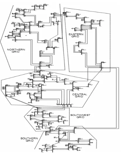
Initially, the work focused on the development of a new dynamic voltage collapse indicator named as the Power Transfer Stability Index (PTSI). The index is calculated by using information of total apparent power of the load, Thevenin voltage and impedance at a bus and the phase angle between Thevenin and load impedance. The value of PTSI will fall between 0 and 1 in which when PTSI value reaches 1, it indicates that a voltage collapse has occurred. Dynamic simulations were carried out for determining the relation between voltage, reactive power and real power at a load bus and the PTSI. Load increase at all the load buses was considered for generating the training and testing data sets. The performance of the proposed SVM technique developed for dynamic voltage stability prediction was evaluated by implementing it on the 87 bus practical power system which is shown in Fig. 1. The performance of the SVM was compared with the MLPNN in order to determine the effectiveness of the SVM in terms of accuracy and computation time in dynamic voltage collapse prediction.

II. DYNAMIC VOLTAGE COLLAPSE INDICATOR

An indicator used for predicting dynamic voltage collapse at a bus is the power transfer stability index (PTSI). The PTSI is calculated by knowing information of the total load power, Thevenin voltage and impedance at a bus and the phase angle between Thevenin and load bus [3]. The formula for the PTSI can be described as,

2 2 _{L Thev} 1 cos

Thev S Z

PTSI

E

E D

(1)

where,

SL : load power at a bus

ȕ : phase angle of the Thevenin impedance ZThev : Thevenin impedance

Į : phase angle of load bus impedance EThev : Thevenin voltage

III. SUPPORT VECTOR MACHINE

Support vector machine (SVM) [9] is gaining popularity due to its many attractive features and promising empirical performance. It adopts the structure risk minimization (SRM) principle which has been shown to be superior to the traditional empirical risk minimization (ERM) principle, employed by conventional neural network. SRM minimizes an upper bound of the generalization error on Vapnik-Chernoverkis dimension, as opposed to ERM that minimizes the training error. This difference equips SVM with good generalization performance, which is the goal of the learning problems. Strong theoretical background provides SVM with global optimal solution and can avoid local minimization. It can solve high-dimension problems with Reproducing Kernel Hilbert Spaces Theory and avoid “dimension disaster”. Now, with the introduction of İ-insensitive loss function, SVM has an advantage in solving nonlinear regression estimation.

Support Vector Regression (SVR)

In SVR, the basic idea is to map the data

x

of the input space into a high dimensional feature space Fvia a nonlinear mapping ĭ and to do linear regression in this space [5]:

( ) , ( )

f x w) x ! b with):Rn oF w, F (2) where,

f x : output function

w : weight vector

x : input

b : bias threshold

< . , . > : dot products in the feature space. Thus, linear regression in a high dimensional feature space

Fcorresponds to nonlinear regression in the low dimensional input space Rn. Since ĭ is fixed, thus w is determined from the finite samples {xi, yi} (i=1,2,3, …, N) by minimizing the sum

of the empirical risk Remp [f] and a complexity term ||w||2,

which enforces flatness in feature space:

> @

> @

2

2 1

, ,

l

reg emp i i i

R f R f O w

¦

LH y f x w O w (3)

where l denotes the sample size, O is regularization constant,

LH is the H-insensitive loss function which is given by,

, ,

0 ( )

( )

for f x y

L y f x w

f x y otherwise

H H

­

° ®

°¯ (4)

The target function (3) can be minimized by solving quadratic programming problem, which is uniquely solvable. It can be normalized as follows:

1 2

, 2

, ,

, 0

i i

i

i i i

i i i

i i

w w C

y w x b

subject to w x b y

[ [ [

H [ H [ [ [

)

­ ) d

°

° _{) d}

® °

t °¯

¦

(5)

where,

C : a pre-specified value

[- _{, [}+ _{: slack variables representing upper and lower}

constraints on the outputs of the system

The first part of this cost function is a weight decay which is used to regulate weight size and penalizes large weights. Due to this regulation, the weight converges to smaller values. Large weights deteriorate the generalization ability of SVM because, usually, they can cause excessive variance. The second part is a penalty function which penalizes errors larger than +H using a so called H-insensitive loss function LH for each of the training points. The positive constant C determines the amount, up to which deviations from H are tolerated. Errors larger than +H are denoted with the so-called slack variables representing values above H ([+) and below H ([-), respectively. The third part of the equation represents constraints that are set to the values of errors between regression prediction ( )f x and true values yi.

The solution is given by,

* *

* * *

, ,

1 1 1

max , max ( ), ( )

2

l l

i i j j i j

i j

W x x

D D D D D D

¦¦

D D D D ) )

*

1

l

i i i i

i

y y

D H D H

¦

(6) With constraints,

*

*

1

0 , , 1,...,

0

i i

l

i i

i

C i l

D D D D d d

¦

(7)

*

1 1 , 2 l

i i i r s

i

w

¦

D D x and b w x x (8)

The Karush-Kuhn-Tucker conditions that are satisfied by the solution are,

*

0, 1,...,

i i i l

D D (9) Therefore, the support vectors are points where exactly one of the Lagrange multipliers are greater than zero (on the boundary), which means that they fulfill the Karush-Kuhn-Tucker condition [10]. Training points with non-zero Lagrange multipliers are called support vectors and give shape to SVR. When

H

0

, we get LHloss function and the optimization problem is simplified as,

1 1 1

1

min ,

2

l l l

i j i j i i

i j i

x x y

E

¦¦

E E

¦

E (10) With constraints, 1 , 1,..., 0 i l i i

C E C i l

E

d d

¦

(11)

and the regression function is given by Equation (2), where

1 1 , 2 l

i i r s

i

w

¦

Ex and b w x x (12) A non-linear mapping can be used to map the data into a high dimensional feature space where linear regression is performed. The Kernel approach is again employed to address the curse of dimensionality. The non-linear SVR solution, using an H-insensitive loss function,

* * * * , , 1 * * 1 1

max , max

1

, 2

l

i i i i i

l l

i i j j i j i j

W y y

K x x

D D D D D D D H D H

D D D D

¦

¦¦

(13) With constraints, * * 1

0 , , 1,...,

0

i i l

i i

i

C i l

D D

D D

d d

¦

(14) Solving Equation (13) with constraints as in Equation (14), determines the Lagrange multipliers, D,D* and the regression function which is given by,

*

( ) _{i i i},

SVs

f x

¦

D D K x x b (15) where,

* 1 * 1 , , 1 , , 2 l

i i i j

i l

i i i r i s

i

w x K x x

b K x x K x x

D D D D

¦

¦

(16)

The support vector equality constraint may be dropped if the Kernel contains a bias term, b being accommodated within the Kernel function. The regression function becomes,

*

1

( ) ,

l

i i i

i

f x

¦

D D K x x (17) In (15) the Kernel function, ( ,k x xi j) )( ), (xi ) xj) . It can be shown that any symmetric Kernel function, k satisfying Mercer’s condition corresponds to a dot product in some feature space [9, 11]. Several Kernel functions are named as Gaussian radial basis function (RBF) Kernel, linear Kernel and multilayer perceptron Kernel. The commonly Kernel function used is the Gaussian RBF Kernel which is written as

2

2

2 ( , )

x y

k x y e V

(18) Note that V2 is a parameter associated with RBF function which has to be tuned.

For prediction cases, any data can be regarded as an input-output system with nonlinear mechanism. Therefore, the support vector machines will essentially build a network which is capable of approximating the underlying functions with acceptable accuracy according to learning samples data.

IV. METHODOLOGY

Before the SVM implementation, time domain simulations considering several contingencies were carried out for the purpose of gathering the training data sets. Simulations were carried out by using the PSS/E commercial software.

A. Data Preprocessing

The training data was obtained by carrying out time domain simulation in which load was increased at every load bus for every second at a certain rate from the base case until the occurrence of a voltage collapse. The training data for each contingency was then recorded. About three hundred training and testing data were generated for use in the SVM and MLPNN.

The selection of input features is an important factor which needs to be considered in the SVM and MLPNN implementation. The input features selected for this work are real and reactive power load (PLoad, QLoad) and the load voltage

and phase angle (VLoad,TLoad). Altogether, there are 224 input

features considered for both SVM and MLPNN.

B. Procedure

The SVM implementation procedure is described as follows:

ii. Generate training and testing data for the SVM, by carrying out simulations considering a) increase loads at all the load buses at a rate of 2% MVA/sec until the system collapse, b) increase loads at individual load buses at a rate of 5% MVA/sec with the loads at the other load buses remaining constant. Measure the voltage, phase angle, real and reactive powers and calculate PTSI at all the load buses

iii. Create a data base for the input vector in the form of [PL,

QL, VL,ș] where PL and QL are the load real and reactive

powers, VL is the voltage magnitude at a load bus and ș

is the voltage phase angle. The target or output vector is in the form of PTSI indices for the corresponding input vector.

iv. For the training data sets, select data sets that give low and high values of PTSI.

v. Select the parameter values of Kernel type and Kernel parameter used for training the SVM.

vi. Train the SVM using the selected training data sets. vii. Repeat steps (v) to (vii) by changing the parameter values

of number of epochs, learning rate and performance goal. viii. Compare results of SVM and MLPNN in terms of computational time and accuracy which is in terms of mean square error (MSE), given as:

2 1

( )

n i i

i

X Y MSE

n

¦

(18) whereXi is output value and Yi is target value.

V. RESULTS AND DISCUSSION

Fig. 1 The 87 bust test system

To evaluate the performance of the SVM in predicting dynamic voltage collapse, a practical 87 bus test system is used for verification of the method. The test system which consists of 23 generators and 56 load buses is shown in Fig. 1. In this study, time domain simulations were carried out using the PSS/E simulation software so as to generate the training data sets. From the simulation results, the PTSI was calculated at every load bus using the power and voltage information. In the SVM training, initially the Kernel function type and Kernel parameter, V were determined by trial and error. The various Kernel types considered for the SVM were the RBF, linear and MLP Kernels [12]. For achieving the required SVM accuracy, the MSE value was chosen to be less than or equal to 0.0003. To investigate the effect of varying the Kernel parameters in determining the SVM accuracy, the values of V were varied according to 0.1, 0.2, 0.5 and 1.0 as shown in Table I.

TABLE I

PERFORMANCE OF KERNEL PARAMETER IN SVM

Kernel Function Type Computational Time (s)

MSE RBF,V = 0.1 13.4164 0.0003 RBF,V = 0.2 10.41 0.0001 RBF,V = 0.5 21.04 0.00009 RBF,V = 1.0 22.24 0.00009 Linear, V = 0.1 83.92 1.10-5 Linear, V = 0.2 41.059 1.10-5 Linear, V = 0.5 69.78 1.10-5 Linear, V = 1.0 81.34 1.10-5 MLP, V = 0.1 5.2335 0.879 MLP, V = 0.2 8.33 0.167 MLP, V = 0.5 7.10 0.093 MLP, V = 1.0 6.80 0.057 It can be seen that by increasing V, the values of MSE decrease for RBF and MLPNN. But for the linear Kernel, the effect of V is not significant because the MSE value remains constant.

In terms of computational time, it can be seen that the MLP kernel is the fastest but it is the least accurate because the MSE value is greater than 0.0001. The performance of the linear Kernel shows that it is most accurate because it gives the smallest MSE, but it has a drawback of long computation time. Comparing the performance of the RBF, linear and MLP Kernels in terms of accuracy and computation time, it can be concluded that the RBF Kernel is the best choice for this SVM because it is accurate (MSE < 0.0003) and it is relatively fast. In this case, the RBF Kernel function type with V = 0.2 is chosen as the parameter for the SVM.

A. Comparison of SVM and MLPNN Results in Dynamic Voltage Collapse Prediction

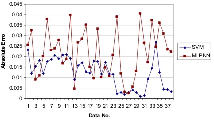
Comparison of SVM and MLPNN for dynamic voltage collapse prediction in terms of absolute errors, the training result for some sampled data is given in Fig. 2. Results show comparison of the SVM and MLPNN absolute error compare to outputs with the actual values of PTSI obtained from simulations.

0 0.005 0.01 0.015 0.02 0.025

1 3 5 7 9 11 13 15 17 19 21 23 25 27 29 31 33 35 37

Data No.

A

b

s

o

lu

te

E

r

r

o

r

SVM MLPNN

Fig. 2 Comparison of absolute error for result training using SVM and MLPNN

Comparison of SVM and MLPNN methods in term of testing result and absolute errors is shown at Fig. 3. Fig. 3 shows the absolute error for training sampled data set for SVM is less than MLPNN.

0 0.005 0.01 0.015 0.02 0.025 0.03 0.035 0.04 0.045

1 3 5 7 9 11 13 15 17 19 21 23 25 27 29 31 33 35 37

Data No.

A

b

s

o

lu

te

E

r

r

o

r

[image:5.595.308.544.86.208.2]

SVM MLPNN

Fig. 3 Comparison of absolute errors for result testing using SVM and MLPNN

[image:5.595.64.278.390.510.2]

The accuracy of the SVM and MLPNN are evaluated based on the absolute errors. The average absolute errors for training and testing of SVM are 0.011 and 0.012 respectively, whilst the average absolute errors for training and testing of MLPNN are 0.01 and 0.021 respectively. The results prove that both the SVM and MLPNN give accurate results in dynamic voltage collapse prediction because the absolute errors are considered small (< 2%). For the purpose of comparing the actual PTSI values obtained from simulations, the PTSI from SVM and PTSI from MLPNN, the PTSI values are plotted as shown in Fig. 4. The results show that in terms of accuracy in predicting dynamic voltage collapse using the PTSI, there is no significant difference between the SVM and MLPNN PTSI values when they arecompared with the actual PTSI values.

Fig. 4 Comparison of actual PTSI, SVM PTSI and MLPNN PTSI

In general, the performance of SVM and MLPNN in predicting dynamic voltage collapse can be evaluated from the results shown in Table II. It can be seen that SVM takes less computational time as compared to MLPNN. In terms of testing accuracy, the MSE for SVM (1.22 x 10-4) is less than MLPNN (2.09 x 10-4). Hence, in general, it can be said that for dynamic voltage collapse prediction, SVM performs better than MLPNN from the speed and accuracy point of views. This feature is particularly important when used in the real-time mode.

TABLE II

PERFORMANCE COMPARISON OF SVM AND MLPNN IN DYNAMIC VOLTAGE COLLAPSE PREDICTION

SVM MLPNN

Training Data 200 200

Testing Data 100 100

Training Error (MSE) 5.84 x 10-4 1 x 10-4 Testing Error (MSE) 1.22 x 10-4 2.09 x 10-4 Computational Time 10.38 s 92 min 30 s

VI. CONCLUSION

Dynamic voltage collapse prediction in power systems using conventional analytical method requires long computational time and therefore to accelerate up the prediction process, SVM approach is proposed. In this study, the SVM is tested for dynamic voltage collapse prediction on a practical 87 bus system. The performance of the SVM method in predicting dynamic voltage collapse based on the PTSI values, is evaluated by comparing it with the MLP NN. In terms of training time, the SVM takes 10.38 secs whereas the MLPNN takes 92 minutes and 30 secs. In terms of accuracy, the SVM using the RBF Kernel function is more accurate than the MLPNN in predicting dynamic voltage collapse for the investigated 87 bus actual power system.

REFERENCES

[1] M. Hasani and M. Parniani, “Method of Combined Static and Dynamic Analysis of Voltage collapse in Voltage Stability Assessment,” IEEE/PES Transmission and Distribution Conference and Exhibition, China, 2005.

[3] M. Nizam, A. Mohamed and A. Hussain, “Performance Evaluation of Voltage Stability Indices for Dynamic Voltage Collapse Prediction”, Journal of Applied Science, vol.6, no.5, pp1104-1113, 2006.

[4] A.W. N. Izzri, A. Mohamed and I. Yahya, “A New Method Of Transient Stability Assessment In Power System Using LS-SVM”, IEEE Student Conference on Research and Development, Malaysia, 11-12 December 2007.

[5] I. Musirin and T.K.A Rahman, 2004, “Voltage stability based weak area clustering technique in power system”, National Power & Energy Conference (PECon 2004), Kuala Lumpur, pp.235-240, 2004. [6] G. Celli, M. Loddo and F. Pilo, “Voltage Collapse Prediction with

Locally Recurrent Neural Network”, International Conference of, pp. 1130-1135, 2002.

[7] S. Krishna and K.R. Padiyar, “Transient Stability Assessment Using Artificial Neural Networks” Proceedings of IEEE International Conference on Industrial Technology, vol.1, pp.627-632, 2000. [8] B. Ravikumar, D. Thukaram and H. P. Khincha, “Application Of

Support Vector Machines For Fault Diagnosis In Power Transmission System,” Generation, Transmission & Distribution, IET, pp. 119-130, 2008.

[9] K. Pelckmans, J. A. K. Suykens, T. Van Gestel, J. De Brabanter, L. Lukas, B. Hamers, B. De Moor and J. Vandewalle, “LS-SVMlab Toolbox User’s Guide,” ESAT-SCD-SISTA Technical Report 02-145, Katholieke Universiteit Leuven, 2003.

[10] A.J. Smola and B. Scholkopf, “On a Kernel-Based Method for Pattern Recognition, Regression, Approximation And Operator Inversion,” Algorithmica, vol.22, pp.211-231, 1998.

[11] D. Z. Gang, N. Lin and Z. J. Guo, “Application of Support Vector Regression Model Based on Phase Space Reconstruction to Power SystemWide-area Stability Prediction”, International Power and Energy Conference (IPEC), Singapore, pp. 1880-1885, 2007.

[12] S. R. Gunn, “Support Vector Machines for Classification and Regression,” Technical Report, Image Speech and Intelligent Systems Research Group, University of Southampton, 1997.

Muhammad Nizam received his B. Elect. Eng. and M. Eng degrees both in Electrical Engineering from Gadjah Mada University, Indonesia in 1994 and in 2002, respectively. Currently, he is Ph.D Student at the Department of Electrical, Electronic and Systems Engineering Department, Universiti Kebangsaan Malaysia. Since 1999, he has been with Engineering Faculty of Sebelas Maret University, Indonesia. His research interests include power system stability and artificial intelligence. He is a student member of IEEE.

Azah Mohamed received her B.Sc from University of London in 1978 and M.Sc and Ph.D from Universiti Malaya in 1988 and 1995, respectively. She is a professor at the Department of Electrical, Electronic and Systems Engineering, Universiti Kebangsaan Malaysia. Her main research interests are in power system security, power quality and artificial intelligence. She is a senior member of IEEE.

Majid Al-Dabbagh graduated with B.Eng. and Master of Technical Science in Engineering from MPEU, Russia, 1968 and obtained his MSc and PhD from UMIST, UK, 1975 and his Grad.Dip.Ed from Melbourne University, Australia, 1991. He was the Head of Electrical and Communication Eng Department, PNG, for 3 years and worked over 24 years at RMIT University, Australia, of which he was the Head of the Electrical Energy and Control Systems Group for over 14 years. He published over 200 papers and edited 5 books and 2 book chapters. He holds Australian and US patents. He is a Chartered Engineer and Fellow of IEE (IET), Chartered Professional Engineer and

Fellow of IEAust, Fellow of the Australian Institute of Energy and a Senior Member of IEEE.