A Mathematical Model For Disease Transmission With Age-structure.

(1)

1

A Mathematical Model for Disease Transmission

with Age-Structure

1

Asep K. Supriatna

Department of Mathematics, Padjadjaran University Km 21 Jatinangor, fax 022-7794696, Sumedang 45363 INDONESIA

Abstract

Many diseases are known to have specific properties, such as one might be easier to transmit to adults while the other might be easier to infect children. For this reason, incorporating age-structure in modelling the disease transmission will give a better insight into how the disease spreads. However, many mathematical models have ignored this age-structure in analysing the disease transmission. In this paper we discuss a simple mathematical model for disease transmission with the inclusion of age-structure. Some classical questions such as the equilibrium population size, the basic reproductive number and the critical vaccination level are investigated. The results show that some properties to some extent are the generalization of the non-age-structure results while some are quite different from the known non-age-non-age-structure results. Keywords: Disease transmission, Age structure, Minimum vaccination level

1. The Model

Suppose that we divide a population into two groups, adults (group 1) and children (group 2). Among the simplest epidemic model in incorporating this division can be done by modifying the simple SIR model described in [1; p.43] to obtain the following equations:

1 1 2 1 12 1 1 11 1

1

B

S

I

S

I

S

dt

dS

µ

β

−

=

, 1

2 2 2 2 22 1 2 21 2

2

B

S

I

S

I

S

dt

dS

µ

β

−

=

, 2

1 1 1 1 2 1 12 1 1 11

1

S

I

S

I

dt

dI

α

µ

β

+

−

=

, 3

2 2 2 2 2 2 22 1 2 21

2

S

I

S

I

dt

dI

α

µ

β

+

−

=

. 4

where S1 and I1 , respectively, denote the numbers of susceptibles and infectives for the adults, and S2 and I2 , respectively, denote the numbers of susceptibles and infectives for the children. Let us assume that the birth rate, mortality rate and recovery rate for each group be Bi,

µ

i and

α

i, respectively. Furthermore, the infection rate in group i is assumed to be proportional to the

1Presented in the International Conference on Statistics and Mathematics and its Application in the Development of Science and Technology, Bandung, October 4-6, 2004. The publication of this paper was funded by the Indonesian Government through the scheme of Penelitian Hibah Bersaing XII (SPK No. 011/P4T/DPPM/PHB/III/2004).

2

numbers of contact between susceptibles in group i and the infectives from groups i and j. Here

ij

β

denotes the constant of proportionality. In the following sections we investigate the effects of mortality rate

µ

_iand infection rate

β

_ijto the equilibrium values

S

_i* and

I

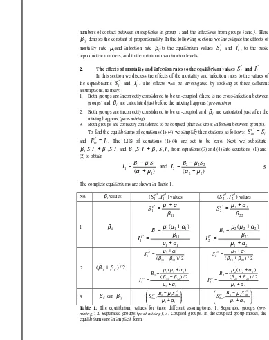
_i*, to the basic reproductive numbers, and to the minimum vaccination levels.

2. The effects of mortality and infection rates to the equilibrium values

S

_i* and

I

*_i

In this section we discuss the effects of the mortality and infection rates to the values of the equilibriums

S

_i* and

I

_i*. The effects will be investigated by looking at three different assumptions, namely:

1. Both groups are incorrectly considered to be un-coupled (there is no cross-infection between groups) and

β

_i are calculated just before the mixing happens (pre-mixing)

2. Both groups are incorrectly considered to be un-coupled and

β

_i are calculated just after the mixing happens (post-mixing)

3. Both groups are correctly considered to be coupled (there is cross-infection between groups). To find the equilibriums of equations (1)-(4) we simplify the notations as follows:

S

_ime*

=

S

_i

and

I

_ime*

=

I

_i_{. The LHS of equations (1)-(4) are set to be zero. Next we substitute} 2

1 12 1 1

11

S

I

β

S

I

β

+

and

β

₂₁

S

₂

I

₁

+

β

₂₂

S

₂

I

₂ from equations (3) and (4) into equations (1) and (2) to obtain

)

(

and

)

(

2 2

2 2 2 2 1 1

1 1 1

1

α

µ

α

µ

+

−

=

+

−

=

B

S

I

B

S

I

. 5

The complete equilibriums are shown in Table 1. No.

β

_ivalues

(

,

*

)

1 * 1

e e

I

S

values

(

,

*

)

2 * 2

e e

I

S

values

1

β

_ii

1 1

11 1 1 1 1 * 1

11 1 1 * 1

)

(

α

µ

β

α

µ

β

α

µ

+

−

=

+

=

B

I

S

e e

2 2

22 2 2 2 2 * 2

22 2 2 * 2

)

(

α

µ

β

α

µ

β

α

µ

+

−

=

+

=

B

I

S

e e

2

(

β +

_ii

β

_ij

)

/

2

1 1

12 11

1 1 1 1 * 1

12 11

1 1 * 1

2 / ) (

) (

2 / ) (

α µ

β β

α µ µ

β β

α µ

+ +

+ − =

+ + =

B I

S

e e

2 2

22 21

2 2 2 2 * 2

22 21

2 2 * 2

2 / ) (

) (

2 / ) (

α µ

β β

α µ µ

β β

α µ

+ +

+ − =

+ + =

B I

S

e e

3

β

ii dan

β

ij 

 

 + −

1 1

* 1 1 1 * 1 ,

α µ

µ e m e

m S B S

  



+ −

2 2

* 2 2 2 * 2 ,

α µ

µ e m e

m S B S

(2)

3

To compare the values of the equilibriums we substitute back the resulting values of

I

₁

and

I

₂ into equations (1) and (2), which were equating to zero beforehand, to obtain

0

)

(

)

(

₂ ₂ 1 1

2 2 2 1 12 1 1

1 1 1 1 11

1

+

−

=

−

+

−

S

B

S

B

S

B

µ

α

µ

β

µ

α

µ

β

, 6

0

)

(

)

(

₂ ₂ 2 2

2 2 2 2 22 1 1

1 1 1 2 21

2

+

−

=

−

+

−

S

B

S

B

S

B

µ

α

µ

β

µ

α

µ

β

. 7

The last two equations were solved (in this case we use Maple V), by considering

α

₁

=

α

₂

=

α

and

B

1

=

B

2

=

B

, to find an implicit form

1 1 2 12

2 2 2

)

(

S

Y

X

S

µ

α

µ

β

+

=

, 8

In which

(

2 1 1 2 11 1 11 2 1 12 1 12 1 1

)

2

B

S

B

S

B

S

B

S

X

=

−

α

+

αµ

+

αµ

+

µ

−

β

α

−

β

µ

−

β

α

−

β

µ

and

(

2

)

1 2 1 11 2 1 1 11 1 2 2 1 1 2 1 1 2 1 1 2 1

2

S

Y

=

−

µ

α

−

αµ

µ

−

αµ

−

µ

+

β

αµ

+

β

µ

.

The expression of

X

₂ can be simplified into

(

₂

)

₁

(

₂

)

₁

(

₁₁ ₁₁ ₂ ₁₂ ₁₂ ₁

)

2

=

−

B

α

+

µ

+

µ

α

+

µ

−

S

β

α

+

β

µ

+

β

α

+

β

µ

X

.

The next simplifications of

X

₂ and

Y

₂ yields

(

₁

)(

₂

)

₁

(

₁₁

(

₂

)

₁₂

(

₁

)

2

=

−

B

α

+

µ

α

+

µ

−

S

β

α

+

µ

+

β

α

+

µ

X

,

9

(

₁

)

₁

(

₂

)

₁₁ ₁ ₁

(

₂

)

1

2

=

−

S

−

α

+

µ

α

+

µ

+

β

N

µ

α

+

µ

Y

.

10 Furthermore, to compare the values of equilibrium of the different groups we let

2

1

S

=

−

∆

, so

1 1 2 12

2 2 1

)

(

S

Y

X

S

µ

α

µ

β

+

−

=

∆

. The RHS can be written as

(

)

(

)

(

)

(

)

(

)

(

)

)(

(

)

(

2 1 1 11 2 1 1 1

1 12 2 11 1 2 1 1

1 2 12 1

µ

α

µ

β

µ

α

µ

α

µ

α

β

µ

α

β

µ

α

µ

α

µ

α

µ

β

+

−

+

−

+

=

S

B

S

)

)(

(

)

)(

(

)

)(

(

1 2 1 1 1 1 2 1 11 2 1 1

12

1

S

B

S

B

S

+

−

+

−

+

−

=

β

α

µ

α

µ

α

µ

β

α

µ

[

(

)(

)

(

)

]

(

)(

)

(

B

−

₁

S

₁

+

₁

+

₂

−

S

₁ ₁₁

+

₂

+

S

₁ ₁₂

+

₁ ₂

S

₁

−

B

=

µ

α

µ

α

µ

β

α

µ

β

α

µ

(

)

[

(

)

(

)

]

(

)(

)

(

B

−

₁

S

₁

+

₂

+

₁

−

S

₁ ₁₁

+

S

₁ ₁₂

+

₁ ₂

S

₁

−

B

=

µ

α

µ

α

µ

β

α

µ

.

It is easy to show that if

µ

₁

=

µ

₂

=

µ

,

β

12

= β

21

=

0

and

β

11

=

β

22

=

β

then

equilibrium values for both groups are equal. The discussion in [2] shows that if

µ ≠

₁

µ

₂ and there are no cross infection between the two group, i.e.

β

₁₂

= β

₂₁

=

0

, then the equilibriums for both groups can be obtained from a single (unstructured) model.

Next we see the following case of

µ ≠

₁

µ

₂ and

β

₁₁

=

β

₁₂

=

β

₂₁

=

β

₂₂

=

β

≠

0

. In this case we assume that the mortality of the two groups are different and each group can infect

4

each other. We will show that S1≠S2. We will also show that conclusion if we incorrectly assume that there is no cross-infection between groups will significantly different from the case if we correctly assume that indeed there is a cross-infection between the groups.

Note that from ∆S=S₁−S₂ we can derive

(

)

[

(

)

(

)

]

(

)(

)

0

)

(

₁ ₁ ₂ ₁ ₁ ₁₁ ₁ ₁₂ ₁ ₂ ₁

2

1

−

S

=

B

−

S

+

−

S

+

S

+

S

−

B

>

S

µ

α

µ

α

µ

β

α

µ

provided

(

B

−

µ

₁

S

₁

)

=

0

and

(

µ

₂

S

₁

−

B

)

>

0

. Alternatively

B

/

S

₁

=

µ

₁ and

B

/

S

₁

<

µ

₂, means that

µ <

₁

µ

₂. This concludes that

µ

₁

< µ

₂

⇒

S

₁

>

S

₂. This result contradicts the result if we incorrectly assume that there is no cross-infection between the groups, that is

* 2 2 1 * 1

e

S

=

+

<

+

=

β

α

µ

β

α

µ

. We give a numerical example to illustrate this phenomenon in [2].

3. The minimum vaccination level

Let us assume that a portion pi of susceptible population is vaccinated so that the dynamics is given by equations (1) to (4) except

i i j i ij i i ii i i

i

p

B

S

I

S

I

S

dt

dS

µ

β

−

=

(

1

)

. 11

Equilibrium values of the system, now are given by

i i

i i vi i i i

vi i

i i

vi i i

i vi i i i vi

R

p

S

B

p

S

B

p

I

α

µ

α

µ

α

µ

+

−

=

+

−

=

+

−

=

(

1

)

1

)

1

(

)

1

(

* ₀

* * * *

, 12

with

* 0 * 0

/

vi i

vi i i i

S

B

R

=

µ

=

. It is clear that eventually there will be no infective if

1

)

1

(

−

p

_i

R

₀_i

≤

means that

i i

R

p

0

1

−

≥

. We conclude that the critical vaccination level for each group is given by

p

_ci

=

1

−

1

/

R

0_i. This value has the same expression as the critical

vaccination level for many known structured or un-structured population models [3].

4. The computation of the basic reproduction ratio

In this section we derive the basic reproductive ratio, R0, for the system in equations (1) to (4). In this system there are two types of infections: type 1 infected by group 1 and type 2 infected by group 2. To find the R0, we construct the next generation matrix









=

22 21

12 11

k

K

where

k

_ij = expected number of new cases of type i infected by one case of type j. Hence,













+

=

j j i ij

ij

S

k

α

µ

β

1

with

S

_idenotes the disease free susceptible equilibrium, i.e i i i

B

S

(3)

5













+

=

2 2

2 22 1 1

2 21

2 2

1 12 1 1

1 11

µ

α

β

µ

α

β

µ

α

β

µ

α

β

S

K

. 13

In [1] it is found that R0 is the dominant eigen value of the matrix K. Since the eigen value for 2x2 matrix is given by the root of the characteristic equation

0

)

(

)

(

2

−

Trace

K

λ

+

Det

K

=

λ

, it can be proved that if

β

_ij

=

a

_i

b

_ithen









+

=

2 2

2 22 1 1

1 11 0

2

1

µ

α

β

µ

α

β

S

R

. 14

In this case R0 for the coupled groups is the average of the R0 for the un-coupled groups. The knowledge of R0 both for coupled or uncoupled groups, and its changes to the change of other parameters, is very important to compare various decisions in controlling the disease. Relevant question regarding an age-structure, such as which group should have a high priority to be vaccinated can be address further. We examine the effects of the mortality and infection rates to the values of R0, and hence to the critical vaccination level, by investigating various cases of

β

ij, elsewhere.

Acknowledgement

The author thanks Prof. E. Soewono of ITB and Prof. J.A.P. Heesterbeek of Utrecht University for the fruitful discussion during the conference excursion in Bali, July 2004. Their views and suggestions have improved the material in the previous draft of this paper. The author also acknowledges the financial support from the Indonesian Government through the scheme of Penelitian Hibah Bersaing XII (SPK No. 011/P4T/DPPM/PHB/III/2004).

References

[1]. Diekmann, O. & J.A.P. Heesterbeek (2000). Mathematical Epidemiology of Infectious Diseases. John Wiley & Son. New York.

[2]. Supriatna, A.K. et al. (2004). Model Metapopulasi Epidemik (In Indonesian). 12th National Conference of Mathematics, Bali 23-27 July 2004.