3
4
5
6
7
8
9
10
11
12
IIIB IVB VB VIB VIIB VIIIB IB IIB
I II III IV V VI VII
VIII
IA IIA IIIA IVA VA VIA VIIA
VIIA
alumin ium silicon phosphorus sulf ur 17chlorine
Cl
18argonAr
26.98 28.09 30.97 32.06 35.45 39.95
30
Zn
31Ga
32Ge
33As
34Se
35Br
36Kr
zinc gallium germa nium arsenic selenium bromine
65.41 69.72 72.64 74.92 78.96 79.90 rubidium st rontium yttrium zirconium niobium molybde num
caesium barium hafnium tantalum tungsten cerium praseodymium neo dymiu m promethium samarium europ iu m gad olinium
thorium protactinium uranium nep tu nium pluton ium americium
terbium dysprosium holmium
berkelium califo rn iu m eins teinium
erbium thulium ytterbium
fermium me ndelev ium nobelium 140.12 140.91 144.24 (145) 150.36 151.96 157.25 158.93
232.04 231.04 238.03 (237) (244) (243) (247) (247)
The elements
Name Symbol Atomic number Molar mass
Sixth Edition
Duward Shriver
Northwestern University
Mark Weller
University of Bath
Tina Overton
University of Hull
Jonathan Rourke
University of Warwick
Fraser Armstrong
University of Oxford
Publisher: Jessica Fiorillo
Associate Director of Marketing: Debbie Clare Associate Editor: Heidi Bamatter
Media Acquisitions Editor: Dave Quinn Marketing Assistant: Samantha Zimbler
Library of Congress Preassigned Control Number: 2013950573
ISBN-13: 978–1–4292–9906–0 ISBN-10: 1–4292–9906–1
©2014, 2010, 2006, 1999 by P.W. Atkins, T.L. Overton, J.P. Rourke, M.T. Weller, and F.A. Armstrong All rights reserved
Published in Great Britain by Oxford University Press
This edition has been authorized by Oxford University Press for sale in the United States and Canada only and not for export therefrom.
First printing
W. H. Freeman and Company 41 Madison Avenue
Preface
Our aim in the sixth edition of Inorganic Chemistry is to provide a comprehensive and contemporary introduction to the diverse and fascinating subject of inorganic chemistry. Inorganic chemistry deals with the properties of all of the elements in the periodic table. These elements range from highly reactive metals, such as sodium, to noble metals, such as gold. The nonmetals include solids, liquids, and gases, and range from the aggressive oxidizing agent fl uorine to unreactive gases such as helium. Although this variety and diversity are features of any study of inorganic chemistry, there are underlying patterns and trends which enrich and enhance our understanding of the discipline. These trends in reactivity, structure, and properties of the elements and their compounds provide an insight into the landscape of the periodic table and provide a foundation on which to build a detailed understanding.
Inorganic compounds vary from ionic solids, which can be described by simple applica-tions of classical electrostatics, to covalent compounds and metals, which are best described by models that have their origin in quantum mechanics. We can rationalize and interpret the properties and reaction chemistries of most inorganic compounds by using qualitative models that are based on quantum mechanics, such as atomic orbitals and their use to form molecular orbitals. Although models of bonding and reactivity clarify and systema-tize the subject, inorganic chemistry is essentially an experimental subject. New inorganic compounds are constantly being synthesized and characterized through research projects especially at the frontiers of the subject, for example, organometallic chemistry, materials chemistry, nanochemistry, and bioinorganic chemistry. The products of this research into inorganic chemistry continue to enrich the fi eld with compounds that give us new perspec-tives on structure, bonding, reactivity, and properties.
Inorganic chemistry has considerable impact on our everyday lives and on other sci-entifi c disciplines. The chemical industry is strongly dependent on it. Inorganic chemistry is essential to the formulation and improvement of modern materials such as catalysts, semiconductors, optical devices, energy generation and storage, superconductors, and advanced ceramics. The environmental and biological impacts of inorganic chemistry are also huge. Current topics in industrial, biological, and sustainable chemistry are men-tioned throughout the book and are developed more thoroughly in later chapters.
In this new edition we have refi ned the presentation, organization, and visual repre-sentation. All of the book has been revised, much has been rewritten, and there is some completely new material. We have written with the student in mind, including some new pedagogical features and enhancing others.
The topics in Part 1, Foundations , have been updated to make them more accessible to
the reader with more qualitative explanation accompanying the more mathematical treat-ments. Some chapters and sections have been expanded to provide greater coverage, par-ticularly where the fundamental topic underpins later discussion of sustainable chemistry.
Part 2, The elements and their compounds , has been substantially strengthened. The
section starts with an enlarged chapter which draws together periodic trends and cross references forward to the descriptive chapters. An enhanced chapter on hydrogen, with reference to the emerging importance of the hydrogen economy, is followed by a series of chapters traversing the periodic table from the s-block metals through the p block to the Group 18 gases. Each of these chapters is organized into two sections: The essentials
describes the fundamental chemistry of the elements and The detail provides a more thor-ough, in-depth account. This is followed by a series of chapters discussing the fascinating chemistry of the d - block and, fi nally, the f-block elements. The descriptions of the chemical
properties of each group of elements and their compounds are enriched with illustrations of current research and applications. The patterns and trends that emerge are rationalized by drawing on the principles introduced in Part 1.
Part 3, Frontiers , takes the reader to the edge of knowledge in several areas of current
Mikhail V. Barybin, University of Kansas Byron L. Bennett, Idaho State University Stefan Bernhard, Carnegie Mellon University
Wesley H. Bernskoetter, Brown University Chris Bradley, Texas Tech University
Thomas C. Brunold, University of Wisconsin – Madison Morris Bullock, Pacifi c Northwest National Laboratory
Gareth Cave, Nottingham Trent University David Clark, Los Alamos National Laboratory
William Connick, University of Cincinnati
Sandie Dann, Loughborough University
Marcetta Y. Darensbourg, Texas A&M University
David Evans, University of Hull Stephen Faulkner, University of Oxford
Bill Feighery, IndianaUniversity – South Bend Katherine J. Franz, Duke University
Carmen Valdez Gauthier, Florida Southern College
Stephen Z. Goldberg, Adelphi University Christian R. Goldsmith, Auburn University
Gregory J. Grant, University of Tennessee at Chattanooga Craig A. Grapperhaus, University of Louisville
P. Shiv Halasyamani, University of Houston Christopher G. Hamaker, Illinois State University
Allen Hill, University of Oxford Andy Holland, Idaho State University Timothy A. Jackson, University of Kansas
Wayne Jones, State University of New York – Binghamton
Deborah Kays, University of Nottingham Susan Killian VanderKam, Princeton University
Michael J. Knapp, University of Massachusetts – Amherst
Georgios Kyriakou, University of Hull
Christos Lampropoulos, University of North Florida
Simon Lancaster, University of East Anglia
John P. Lee, University of Tennessee at Chattanooga
Ramón López de la Vega, Florida International University Yi Lu, University of Illinois at Urbana-Champaign
Joel T. Mague, Tulane University
Andrew Marr, Queen’s University Belfast
Salah S. Massoud, University of Louisiana at Lafayette
Charles A. Mebi, Arkansas Tech University Catherine Oertel, Oberlin College
Jason S. Overby, College of Charleston John R. Owen, University of Southampton
Ted M. Pappenfus, University of Minnesota, Morris
Anna Peacock, University of Birmingham Carl Redshaw, University of Hull
Laura Rodríguez Raurell, University of Barcelona
Professor Jean-Michel Savéant, Université Paris Diderot – Paris 7
Douglas L. Swartz II, Kutztown University of Pennsylvania Jesse W. Tye, Ball State University
Derek Wann, University of Edinburgh Scott Weinert, Oklahoma State University
Nathan West, University of the Sciences
Denyce K. Wicht, Suffolk University
Acknowledgments
About the book
Inorganic Chemistry provides numerous learning features to help you master this
wide-ranging subject. In addition, the text has been designed so that you can either work through the chapters chronologically, or dip in at an appropriate point in your studies. The text’s Book Companion Site provides further electronic resources to support you in your learning.
The material in this book has been logically and systematically laid out, in three dis-tinct sections. Part 1, Foundations, outlines the underlying principles of inorganic
chem-istry, which are built on in the subsequent two sections. Part 2, The elements and their
compounds, divides the descriptive chemistry into ‘essentials’ and ‘detail’, enabling you to
easily draw out the key principles behind the reactions, before exploring them in greater depth. Part 3, Frontiers, introduces you to exciting interdisciplinary research at the
fore-front of inorganic chemistry.
The paragraphs below describe the learning features of the text and Book Companion Site in further detail.
Organizing the information
Key points
The key points outline the main take-home message(s) of the section that follows. These will help you to focus on the prin-cipal ideas being introduced in the text.
Context boxes
Context boxes demonstrate the diversity of inorganic chem-istry and its wide-ranging applications to, for example, advanced materials, industrial processes, environmental chemistry, and everyday life.
Further reading
Each chapter lists sources where further information can be found. We have tried to ensure that these sources are easily available and have indicated the type of information each one provides.
Resource section
At the back of the book is a comprehensive collection of resources, including an extensive data section and informa-tion relating to group theory and spectroscopy.
Notes on good practice
ix
About the bookProblem solving
Brief illustrations
A Brief illustration shows you how to use equations or
con-cepts that have just been introduced in the main text, and will help you to understand how to manipulate data correctly.
Worked examples and Self-tests
Numerous worked Examples provide a more detailed illustra-tion of the applicaillustra-tion of the material being discussed. Each one demonstrates an important aspect of the topic under dis-cussion or provides practice with calculations and problems. Each Example is followed by a Self-test designed to help you monitor your progress.
Exercises
There are many brief Exercises at the end of each chapter. You can fi nd the answers on the Book Companion Site and fully worked solutions are available in the separate Solutions man-ual . The Exercises can be used to check your understanding and gain experience and practice in tasks such as balancing equa-tions, predicting and drawing structures, and manipulating data .
Tutorial Problems
The Tutorial Problems are more demanding in content and
style than the Exercises and are often based on a research paper or other additional source of information. Problem questions generally require a discursive response and there may not be a single correct answer. They may be used as essay type ques-tions or for classroom discussion.
Solutions Manual
Book Companion Site
The Book Companion Site to accompany this book provides a number of useful teaching and learning resources to augment the printed book, and is free of charge.
The site can be accessed at: www.whfreeman.com/ichem6e
Please note that instructor resources are available only to registered adopters of the text-book. To register, simply visit www.whfreeman.com/ichem6e and follow the appropriate links.
Student resources are openly available to all, without registration.
Materials on the Book Companion Site include:
3D rotatable molecular structures
Numbered structures can be found online as interactive 3D
struc-tures. Type the following URL into your browser, adding the rel-evant structure number: www.chemtube3d.com/weller/ [chapter number]S[structure number]. For example, for structure 10 in Chapter 1, type www.chemtube3d.com/weller/1S10 .
Those fi gures with an asterisk (*) in the caption can also be
found online as interactive 3D structures. Type the following URL into your browser, adding the relevant fi gure number: www. chemtube3d.com/weller/ [chapter number]F[fi gure number]. For example, for Figure 4 in chapter 7, type www.chemtube3d.com/ weller/7F04 .
Visit www.chemtube3d.com/weller/ [chapter number] for all 3D resources organized by chapter.
Answers to Self-tests and Exercises
There are many Self-tests throughout each chapter and brief
Exercises at the end of each chapter. You can fi nd the answers on
the Book Companion Site.
Videos of chemical reactions
Video clips showing demonstrations of a variety of inorganic chemistry reactions are avail-able for certain chapters of the book.
Molecular modeling problems
Molecular modeling problems are available for almost every chapter, and are written to be performed using the popular Spartan Student TM software. However, they can also be completed using any electronic structure program that allows Hartree–Fock, density func-tional, and MP2 calculations.
Group theory tables
xi
Book Companion SiteFor registered adopters:
Figures and tables from the book
Summary of contents
Part 1
Foundations
11 Atomic structure 3
2 Molecular structure and bonding 34
3 The structures of simple solids 65
4 Acids and bases 116
5 Oxidation and reduction 154
6 Molecular symmetry 188
7 An introduction to coordination compounds 209
8 Physical techniques in inorganic chemistry 234
Part 2
The elements and their compounds
2719 Periodic trends 273
10 Hydrogen 296
11 The Group 1 elements 318
12 The Group 2 elements 336
13 The Group 13 elements 354
14 The Group 14 elements 381
15 The Group 15 elements 408
16 The Group 16 elements 433
17 The Group 17 elements 456
18 The Group 18 elements 479
19 The d-block elements 488
20 d-Metal complexes: electronic structure and properties 515
21 Coordination chemistry: reactions of complexes 550
22 d-Metal organometallic chemistry 579
23 The f-block elements 625
Part 3
Frontiers
65324 Materials chemistry and nanomaterials 655
25 Catalysis 728
26 Biological inorganic chemistry 763
27 Inorganic chemistry in medicine 820
Resource section 1: Selected ionic radii 834
Resource section 2: Electronic properties of the elements 836
Resource section 3: Standard potentials 838
Resource section 4: Character tables 851
Resource section 5: Symmetry-adapted orbitals 856
Resource section 6: Tanabe–Sugano diagrams 860
Contents
Glossary of chemical abbreviations xxi
Part 1
Foundations
11 Atomic structure 3
The structures of hydrogenic atoms 4
1.1 Spectroscopic information 6
1.2 Some principles of quantum mechanics 8
1.3 Atomic orbitals 9
Many-electron atoms 15
1.4 Penetration and shielding 15
1.5 The building-up principle 17
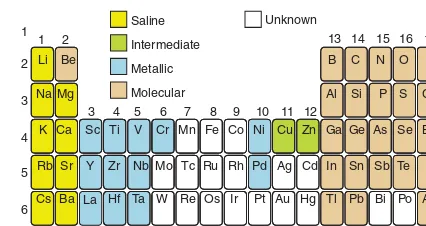
1.6 The classifi cation of the elements 20
1.7 Atomic properties 22
FURTHER READING 32
EXERCISES 32
TUTORIAL PROBLEMS 33
2 Molecular structure and bonding 34
Lewis structures 34
2.1 The octet rule 34
2.2 Resonance 35
2.3 The VSEPR model 36
Valence bond theory 39
2.4 The hydrogen molecule 39
2.5 Homonuclear diatomic molecules 40
2.6 Polyatomic molecules 40
Molecular orbital theory 42
2.7 An introduction to the theory 43 2.8 Homonuclear diatomic molecules 45 2.9 Heteronuclear diatomic molecules 48
2.10 Bond properties 50
2.11 Polyatomic molecules 52
2.12 Computational methods 56
Structure and bond properties 58
2.13 Bond length 58
2.14 Bond strength 58
2.15 Electronegativity and bond enthalpy 59
2.16 Oxidation states 61
FURTHER READING 62
EXERCISES 62
TUTORIAL PROBLEMS 63
3 The structures of simple solids 65
The description of the structures of solids 66 3.1 Unit cells and the description of crystal structures 66 3.2 The close packing of spheres 69 3.3 Holes in close-packed structures 70
The structures of metals and alloys 72
3.4 Polytypism 73
3.5 Nonclose-packed structures 74
3.6 Polymorphism of metals 74
3.7 Atomic radii of metals 75
3.8 Alloys and interstitials 76
Ionic solids 80
3.9 Characteristic structures of ionic solids 80 3.10 The rationalization of structures 87
The energetics of ionic bonding 91
3.11 Lattice enthalpy and the Born–Haber cycle 91 3.12 The calculation of lattice enthalpies 93 3.13 Comparison of experimental and theoretical values 95 3.14 The Kapustinskii equation 97 3.15 Consequences of lattice enthalpies 98
Defects and nonstoichiometry 102
3.16 The origins and types of defects 102 3.17 Nonstoichiometric compounds and solid solutions 105
The electronic structures of solids 107
3.18 The conductivities of inorganic solids 107 3.19 Bands formed from overlapping atomic orbitals 107
3.20 Semiconduction 110
FURTHER INFORMATION: the Born–Mayer equation 112
FURTHER READING 113
EXERCISES 113
TUTORIAL PROBLEMS 115
4 Acids and bases 116
Brønsted acidity 117
4.1 Proton transfer equilibria in water 117
Characteristics of Brønsted acids 125
4.2 Periodic trends in aqua acid strength 126
4.3 Simple oxoacids 126
4.4 Anhydrous oxides 129
4.5 Polyoxo compound formation 130
Lewis acidity 132
Reactions and properties of Lewis acids and bases 137 4.8 The fundamental types of reaction 137 4.9 Factors governing interactions between Lewis
acids and bases 139
4.10 Thermodynamic acidity parameters 141
Nonaqueous solvents 142
4.11 Solvent levelling 142
4.12 The solvent-system defi nition of acids and bases 144 4.13 Solvents as acids and bases 145
Applications of acid–base chemistry 149
4.14 Superacids and superbases 149 4.15 Heterogeneous acid–base reactions 150
FURTHER READING 151
EXERCISES 151
TUTORIAL PROBLEMS 153
5 Oxidation and reduction 154
Reduction potentials 155
5.1 Redox half-reactions 155
5.2 Standard potentials and spontaneity 156 5.3 Trends in standard potentials 160 5.4 The electrochemical series 161
5.5 The Nernst equation 162
Redox stability 164
5.6 The infl uence of pH 164
5.7 Reactions with water 165
5.8 Oxidation by atmospheric oxygen 166 5.9 Disproportionation and comproportionation 167 5.10 The infl uence of complexation 168 5.11 The relation between solubility and standard potentials 170 Diagrammatic presentation of potential data 170
5.12 Latimer diagrams 171
5.13 Frost diagrams 173
5.14 Pourbaix diagrams 177
5.15 Applications in environmental chemistry: natural waters 177
Chemical extraction of the elements 178
5.16 Chemical reduction 178
5.17 Chemical oxidation 182
5.18 Electrochemical extraction 183
FURTHER READING 184
EXERCISES 185
TUTORIAL PROBLEMS 186
6 Molecular symmetry 188
An introduction to symmetry analysis 188
6.1 Symmetry operations, elements, and point groups 188
6.2 Character tables 193
Applications of symmetry 196
6.3 Polar molecules 196
6.4 Chiral molecules 196
6.5 Molecular vibrations 197
The symmetries of molecular orbitals 201
6.6 Symmetry-adapted linear combinations 201 6.7 The construction of molecular orbitals 203 6.8 The vibrational analogy 204
Representations 205
6.9 The reduction of a representation 205
6.10 Projection operators 207
FURTHER READING 208
EXERCISES 208
TUTORIAL PROBLEMS 208
7 An introduction to coordination compounds 209
The language of coordination chemistry 210
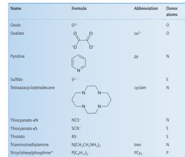
7.1 Representative ligands 210
7.2 Nomenclature 212
Constitution and geometry 214
7.3 Low coordination numbers 214 7.4 Intermediate coordination numbers 215 7.5 Higher coordination numbers 216
7.6 Polymetallic complexes 218
Isomerism and chirality 218
7.7 Square-planar complexes 219
7.8 Tetrahedral complexes 220
7.9 Trigonal-bipyramidal and square-pyramidal complexes 220
7.10 Octahedral complexes 221
7.11 Ligand chirality 224
The thermodynamics of complex formation 225
7.12 Formation constants 226
7.13 Trends in successive formation constants 227 7.14 The chelate and macrocyclic effects 229 7.15 Steric effects and electron delocalization 229
FURTHER READING 231
EXERCISES 231
TUTORIAL PROBLEMS 232
8 Physical techniques in inorganic chemistry 234
Diffraction methods 234
8.1 X-ray diffraction 234
8.2 Neutron diffraction 238
Absorption and emission spectroscopies 239
xv
ContentsResonance techniques 247
8.6 Nuclear magnetic resonance 247 8.7 Electron paramagnetic resonance 252
8.8 Mössbauer spectroscopy 254
Ionization-based techniques 255
8.9 Photoelectron spectroscopy 255 8.10 X-ray absorption spectroscopy 256
8.11 Mass spectrometry 257
Chemical analysis 259
8.12 Atomic absorption spectroscopy 260
8.13 CHN analysis 260
8.14 X-ray fl uorescence elemental analysis 261
8.15 Thermal analysis 262
Magnetometry and magnetic susceptibility 264
Electrochemical techniques 264
Microscopy 266
8.16 Scanning probe microscopy 266
8.17 Electron microscopy 267
FURTHER READING 268
EXERCISES 268
TUTORIAL PROBLEMS 269
Part 2
The elements and their compounds
2719 Periodic trends 273
Periodic properties of the elements 273
9.1 Valence electron confi gurations 273
9.2 Atomic parameters 274
9.3 Occurrence 279
9.4 Metallic character 280
9.5 Oxidation states 281
Periodic characteristics of compounds 285
9.6 Coordination numbers 285
9.7 Bond enthalpy trends 285
9.8 Binary compounds 287
9.9 Wider aspects of periodicity 289 9.10 Anomalous nature of the fi rst member of each group 293
FURTHER READING 295
EXERCISES 295
TUTORIAL PROBLEMS 295
10 Hydrogen 296
Part A: The essentials 296
10.1 The element 297
10.2 Simple compounds 298
Part B: The detail 302
10.3 Nuclear properties 302
10.4 Production of dihydrogen 303
10.5 Reactions of dihydrogen 305
10.6 Compounds of hydrogen 306
10.7 General methods for synthesis of binary hydrogen
compounds 315
FURTHER READING 316
EXERCISES 316
TUTORIAL PROBLEMS 317
11 The Group 1 elements 318
Part A: The essentials 318
11.1 The elements 318
11.2 Simple compounds 320
11.3 The atypical properties of lithium 321
Part B: The detail 321
11.4 Occurrence and extraction 321 11.5 Uses of the elements and their compounds 322
11.6 Hydrides 324
11.7 Halides 324
11.8 Oxides and related compounds 326 11.9 Sulfi des, selenides, and tellurides 327
11.10 Hydroxides 327
11.11 Compounds of oxoacids 328
11.12 Nitrides and carbides 330
11.13 Solubility and hydration 330 11.14 Solutions in liquid ammonia 331 11.15 Zintl phases containing alkali metals 331
11.16 Coordination compounds 332
11.17 Organometallic compounds 333
FURTHER READING 334
EXERCISES 334
TUTORIAL PROBLEMS 334
12 The Group 2 elements 336
Part A: The essentials 336
12.1 The elements 336
12.2 Simple compounds 337
12.3 The anomalous properties of beryllium 339
Part B: The detail 339
12.4 Occurrence and extraction 339 12.5 Uses of the elements and their compounds 340
12.6 Hydrides 342
12.7 Halides 343
12.8 Oxides, sulfi des, and hydroxides 344
12.9 Nitrides and carbides 346
12.11 Solubility, hydration, and beryllates 349
12.12 Coordination compounds 349
12.13 Organometallic compounds 350
FURTHER READING 352
EXERCISES 352
TUTORIAL PROBLEMS 352
13 The Group 13 elements 354
Part A: The essentials 354
13.1 The elements 354
13.2 Compounds 356
13.3 Boron clusters 359
Part B: The detail 359
13.4 Occurrence and recovery 359
13.5 Uses of the elements and their compounds 360 13.6 Simple hydrides of boron 361
13.7 Boron trihalides 363
13.8 Boron–oxygen compounds 364
13.9 Compounds of boron with nitrogen 365
13.10 Metal borides 366
13.11 Higher boranes and borohydrides 367 13.12 Metallaboranes and carboranes 372 13.13 The hydrides of aluminium and gallium 374 13.14 Trihalides of aluminium, gallium, indium, and thallium 374 13.15 Low-oxidation-state halides of aluminium, gallium,
indium, and thallium 375
13.16 Oxo compounds of aluminium, gallium, indium,
and thallium 376
13.17 Sulfi des of gallium, indium, and thallium 376 13.18 Compounds with Group 15 elements 376
13.19 Zintl phases 377
13.20 Organometallic compounds 377
FURTHER READING 378
EXERCISES 378
TUTORIAL PROBLEMS 379
14 The Group 14 elements 381
Part A: The essentials 381
14.1 The elements 381
14.2 Simple compounds 383
14.3 Extended silicon–oxygen compounds 385
Part B: The detail 385
14.4 Occurrence and recovery 385
14.5 Diamond and graphite 386
14.6 Other forms of carbon 387
14.7 Hydrides 390
14.8 Compounds with halogens 392
14.9 Compounds of carbon with oxygen and sulfur 394
14.10 Simple compounds of silicon with oxygen 396 14.11 Oxides of germanium, tin, and lead 397 14.12 Compounds with nitrogen 398
14.13 Carbides 398
14.14 Silicides 401
14.15 Extended silicon–oxygen compounds 401 14.16 Organosilicon and organogermanium compounds 404 14.17 Organometallic compounds 405
FURTHER READING 406
EXERCISES 406
TUTORIAL PROBLEMS 407
15 The Group 15 elements 408
Part A: The essentials 408
15.1 The elements 409
15.2 Simple compounds 410
15.3 Oxides and oxanions of nitrogen 411
Part B: The detail 411
15.4 Occurrence and recovery 411
15.5 Uses 412
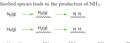
15.6 Nitrogen activation 414
15.7 Nitrides and azides 415
15.8 Phosphides 416
15.9 Arsenides, antimonides, and bismuthides 417
15.10 Hydrides 417
15.11 Halides 419
15.12 Oxohalides 420
15.13 Oxides and oxoanions of nitrogen 421 15.14 Oxides of phosphorus, arsenic, antimony, and bismuth 425 15.15 Oxoanions of phosphorus, arsenic, antimony, and bismuth 425
15.16 Condensed phosphates 427
15.17 Phosphazenes 428
15.18 Organometallic compounds of arsenic, antimony,
and bismuth 428
FURTHER READING 430
EXERCISES 430
TUTORIAL PROBLEMS 431
16 The Group 16 elements 433
Part A: The essentials 433
16.1 The elements 433
16.2 Simple compounds 435
16.3 Ring and cluster compounds 437
Part B: The detail 438
16.4 Oxygen 438
16.5 Reactivity of oxygen 439
16.6 Sulfur 440
xvii
Contents16.8 Hydrides 441
16.9 Halides 444
16.10 Metal oxides 445
16.11 Metal sulfi des, selenides, tellurides, and polonides 445
16.12 Oxides 447
16.13 Oxoacids of sulfur 449
16.14 Polyanions of sulfur, selenium, and tellurium 452 16.15 Polycations of sulfur, selenium, and tellurium 452 16.16 Sulfur–nitrogen compounds 453
FURTHER READING 454
EXERCISES 454
TUTORIAL PROBLEMS 455
17 The Group 17 elements 456
Part A: The essentials 456
17.1 The elements 456
17.2 Simple compounds 458
17.3 The interhalogens 460
Part B: The detail 461
17.4 Occurrence, recovery, and uses 461 17.5 Molecular structure and properties 463
17.6 Reactivity trends 464
17.7 Pseudohalogens 465
17.8 Special properties of fl uorine compounds 466
17.9 Structural features 466
17.10 The interhalogens 467
17.11 Halogen oxides 470
17.12 Oxoacids and oxoanions 471
17.13 Thermodynamic aspects of oxoanion redox reactions 472 17.14 Trends in rates of oxoanion redox reactions 473 17.15 Redox properties of individual oxidation states 474
17.16 Fluorocarbons 475
FURTHER READING 476
EXERCISES 476
TUTORIAL PROBLEMS 478
18 The Group 18 elements 479
Part A: The essentials 479
18.1 The elements 479
18.2 Simple compounds 480
Part B: The detail 481
18.3 Occurrence and recovery 481
18.4 Uses 481
18.5 Synthesis and structure of xenon fl uorides 482 18.6 Reactions of xenon fl uorides 482
18.7 Xenon–oxygen compounds 483
18.8 Xenon insertion compounds 484
18.9 Organoxenon compounds 484
18.10 Coordination compounds 485
18.11 Other compounds of noble gases 486
FURTHER READING 486
EXERCISES 486
TUTORIAL PROBLEMS 487
19 The d-block elements 488
Part A: The essentials 488
19.1 Occurrence and recovery 488 19.2 Chemical and physical properties 489
Part B: The detail 491
19.3 Group 3: scandium, yttrium, and lanthanum 491 19.4 Group 4: titanium, zirconium, and hafnium 493 19.5 Group 5: vanadium, niobium, and tantalum 494 19.6 Group 6: chromium, molybdenum, and tungsten 498 19.7 Group 7: manganese, technetium, and rhenium 502 19.8 Group 8: iron, ruthenium, and osmium 504 19.9 Group 9: cobalt, rhodium, and iridium 506 19.10 Group 10: nickel, palladium, and platinum 507 19.11 Group 11: copper, silver, and gold 508 19.12 Group 12: zinc, cadmium, and mercury 510
FURTHER READING 513
EXERCISES 514
TUTORIAL PROBLEMS 514
20 d-Metal complexes: electronic structure
and properties 515
Electronic structure 515
20.1 Crystal-fi eld theory 515
20.2 Ligand-fi eld theory 525
Electronic spectra 530
20.3 Electronic spectra of atoms 530 20.4 Electronic spectra of complexes 536
20.5 Charge-transfer bands 540
20.6 Selection rules and intensities 541
20.7 Luminescence 543
Magnetism 544
20.8 Cooperative magnetism 544
20.9 Spin-crossover complexes 546
FURTHER READING 547
EXERCISES 547
TUTORIAL PROBLEMS 548
21 Coordination chemistry: reactions of complexes 550
Ligand substitution reactions 550
Ligand substitution in square-planar complexes 555 21.3 The nucleophilicity of the entering group 556 21.4 The shape of the transition state 557
Ligand substitution in octahedral complexes 560 21.5 Rate laws and their interpretation 560 21.6 The activation of octahedral complexes 562
21.7 Base hydrolysis 565
21.8 Stereochemistry 566
21.9 Isomerization reactions 567
Redox reactions 568
21.10 The classifi cation of redox reactions 568 21.11 The inner-sphere mechanism 568 21.12 The outer-sphere mechanism 570
Photochemical reactions 574
21.13 Prompt and delayed reactions 574 21.14 d–d and charge-transfer reactions 574 21.15 Transitions in metal–metal bonded systems 576
FURTHER READING 576
EXERCISES 576
TUTORIAL PROBLEMS 577
22 d-Metal organometallic chemistry 579
Bonding 580
22.1 Stable electron confi gurations 580 22.2 Electron-count preference 581 22.3 Electron counting and oxidation states 582
22.4 Nomenclature 584
Ligands 585
22.5 Carbon monoxide 585
22.6 Phosphines 587
22.7 Hydrides and dihydrogen complexes 588 22.8 η1 -Alkyl, -alkenyl, -alkynyl, and -aryl ligands 589 22.9 η2 -Alkene and -alkyne ligands 590 22.10 Nonconjugated diene and polyene ligands 591 22.11 Butadiene, cyclobutadiene, and cyclooctatetraene 591 22.12 Benzene and other arenes 593
22.13 The allyl ligand 594
22.14 Cyclopentadiene and cycloheptatriene 595
22.15 Carbenes 597
22.16 Alkanes, agostic hydrogens, and noble gases 597 22.17 Dinitrogen and nitrogen monoxide 598
Compounds 599
22.18 d-Block carbonyls 599
22.19 Metallocenes 606
22.20 Metal–metal bonding and metal clusters 610
Reactions 614
22.21 Ligand substitution 614
22.22 Oxidative addition and reductive elimination 617
22.23 σ-Bond metathesis 619
22.24 1,1-Migratory insertion reactions 619 22.25 1,2-Insertions and β-hydride elimination 620 22.26 α-, γ-, and δ-Hydride eliminations and cyclometallations 621
FURTHER READING 622
EXERCISES 622
TUTORIAL PROBLEMS 623
23 The f-block elements 625
The elements 626
23.1 The valence orbitals 626
23.2 Occurrence and recovery 627
23.3 Physical properties and applications 627
Lanthanoid chemistry 628
23.4 General trends 628
23.5 Electronic, optical, and magnetic properties 632
23.6 Binary ionic compounds 636
23.7 Ternary and complex oxides 638
23.8 Coordination compounds 639
23.9 Organometallic compounds 641
Actinoid chemistry 643
23.10 General trends 643
23.11 Electronic spectra of the actinoids 647
23.12 Thorium and uranium 648
23.13 Neptunium, plutonium, and americium 649
FURTHER READING 650
EXERCISES 650
TUTORIAL PROBLEMS 651
Part 3
Frontiers
65324 Materials chemistry and nanomaterials 655
Synthesis of materials 656
24.1 The formation of bulk material 656
Defects and ion transport 659
24.2 Extended defects 659
24.3 Atom and ion diffusion 660
24.4 Solid electrolytes 661
Metal oxides, nitrides, and fl uorides 665
24.5 Monoxides of the 3d metals 665 24.6 Higher oxides and complex oxides 667
24.7 Oxide glasses 676
24.8 Nitrides, fl uorides, and mixed-anion phases 679
xix
Hydrides and hydrogen-storage materials 694
24.13 Metal hydrides 694
24.14 Other inorganic hydrogen-storage materials 696
Optical properties of inorganic materials 696
24.15 Coloured solids 697
24.16 White and black pigments 698
24.17 Photocatalysts 699
Semiconductor chemistry 700
24.18 Group 14 semiconductors 701 24.19 Semiconductor systems isoelectronic with silicon 702
Molecular materials and fullerides 703
24.20 Fullerides 703
Nanostructures and properties 713
24.27 One-dimensional control: carbon nanotubes
and inorganic nanowires 713
24.28 Two-dimensional control: graphene, quantum wells,
Heterogeneous catalysis 742
25.10 The nature of heterogeneous catalysts 743
25.11 Hydrogenation catalysts 747
25.12 Ammonia synthesis 748
25.13 Sulfur dioxide oxidation 749 25.14 Catalytic cracking and the interconversion of aromatics
by zeolites 749
27 Inorganic chemistry in medicine 820
The chemistry of elements in medicine 820
27.1 Inorganic complexes in cancer treatment 821
27.2 Anti-arthritis drugs 824
27.3 Bismuth in the treatment of gastric ulcers 825 27.4 Lithium in the treatment of bipolar disorders 826 27.5 Organometallic drugs in the treatment of malaria 826 27.6 Cyclams as anti-HIV agents 827 27.7 Inorganic drugs that slowly release CO: an agent
against post-operative stress 828
27.8 Chelation therapy 828
27.9 Imaging agents 830
27.10 Outlook 832
FURTHER READING 832
EXERCISES 833
TUTORIAL PROBLEMS 833
Resource sections 834
Resource section 1: Selected ionic radii 834 Resource section 2: Electronic properties of the elements 836 Resource section 3: Standard potentials 838 Resource section 4: Character tables 851 Resource section 5: Symmetry-adapted orbitals 856 Resource section 6: Tanabe–Sugano diagrams 860
Glossary of chemical abbreviations
Ac acetyl, CH 3 CO acac acetylacetonato
aq aqueous solution species bpy 2,2′-bipyridine
cod 1,5-cyclooctadiene cot cyclooctatetraene Cy cyclohexyl Cp cyclopentadienyl
Cp* pentamethylcyclopentadienyl cyclam tetraazacyclotetradecane dien diethylenetriamine DMSO dimethylsulfoxide DMF dimethylformamide
η hapticity
edta ethylenediaminetetraacetato
en ethylenediamine (1,2-diaminoethane) Et ethyl
gly glycinato Hal halide
i Pr isopropyl
L a ligand
μ signifi es a bridging ligand M a metal
Me methyl
mes mesityl, 2,4,6-trimethylphenyl Ox an oxidized species
ox oxalato Ph phenyl phen phenanthroline py pyridine Red a reduced species
Sol solvent, or a solvent molecule soln nonaqueous solution species
t Bu tertiary butyl
THF tetrahydrofuran
TMEDA N , N ,N′, N′-tetramethylethylenediamine trien 2,2′,2″-triaminotriethylene
PART 1
Foundations
The structures of hydrogenic atoms
1.1 Spectroscopic information 1.2 Some principles of quantum
mechanics 1.3 Atomic orbitals
Many-electron atoms
1.4 Penetration and shielding 1.5 The building-up principle 1.6 The classifi cation of the elements 1.7 Atomic properties
Further reading
Exercises
Tutorial problems This chapter lays the foundations for the explanation of the trends in the physical and chemical
properties of all inorganic compounds. To understand the behaviour of molecules and solids we need to understand atoms: our study of inorganic chemistry must therefore begin with a review of their structures and properties. We start with a discussion of the origin of matter in the solar system and then consider the development of our understanding of atomic structure and the behaviour of electrons in atoms. We introduce quantum theory qualitatively and use the results to rationalize properties such as atomic radii, ionization energy, electron affi nity, and electronegativ-ity. An understanding of these properties allows us to begin to rationalize the diverse chemical properties of the more than 110 elements known today.
The observation that the universe is expanding has led to the current view that about 14 billion years ago the currently visible universe was concentrated into a point-like region that exploded in an event called the Big Bang . With initial temperatures immediately after
the Big Bang of about 10 9 K, the fundamental particles produced in the explosion had too much kinetic energy to bind together in the forms we know today. However, the universe cooled as it expanded, the particles moved more slowly, and they soon began to adhere together under the infl uence of a variety of forces. In particular, the strong force , a
short-range but powerful attractive force between nucleons (protons and neutrons), bound these particles together into nuclei. As the temperature fell still further, the electromagnetic
force , a relatively weak but long-range force between electric charges, bound electrons to
nuclei to form atoms, and the universe acquired the potential for complex chemistry and the existence of life ( Box 1.1 ).
About two hours after the start of the universe, the temperature had fallen so much that most of the matter was in the form of H atoms (89 per cent) and He atoms (11 per cent). In one sense, not much has happened since then for, as Fig. 1.1 shows, hydrogen and helium remain overwhelmingly the most abundant elements in the universe. However, nuclear reactions have formed a wide assortment of other elements and have immeasur-ably enriched the variety of matter in the universe, and thus given rise to the whole area of chemistry ( Boxes 1.2 and 1.3 ).
Table 1.1 summarizes the properties of the subatomic particles that we need to sider in chemistry. All the known elements—by 2012, 114, 116, and 118 had been con-fi rmed, although not 115 or 117, and several more are candidates for concon-fi rmation—that are formed from these subatomic particles are distinguished by their atomic number , Z ,
the number of protons in the nucleus of an atom of the element. Many elements have a number of isotopes , which are atoms with the same atomic number but different atomic masses. These isotopes are distinguished by the mass number , A , which is the total number
of protons and neutrons in the nucleus. The mass number is also sometimes termed more appropriately the nucleon number . Hydrogen, for instance, has three isotopes. In each
1
Atomic structure
Those fi gures with an asterisk (*) in the caption can be found online as interactive 3D structures. Type the following URL into your browser, adding the relevant fi gure number: www.chemtube3d.com/weller/[chapter number]F[fi gure number]. For example, for Figure 4 in chapter 7, type www.chemtube3d.com/weller/7F04.
B OX 1.1 Nucleosynthesis of the elements
The earliest stars resulted from the gravitational condensation of clouds of H and He atoms. This gave rise to high temperatures and densities within them, and fusion reactions began as nuclei merged together.
Energy is released when light nuclei fuse together to give elements of higher atomic number. Nuclear reactions are very much more energetic than normal chemical reactions because the strong force which binds protons and neutrons together is much stronger than the electromagnetic force that binds electrons to nuclei. Whereas a typical chemical reaction might release about 10 3 kJ mol −1 , a nuclear reaction typically releases a million times more energy, about 10 9 kJ mol −1 .
Elements up to Z = 26 were formed inside stars. Such elements are the products of the nuclear fusion reactions referred to as ‘nuclear burning’. The burning reactions, which should not be confused with chemical combus-tion, involved H and He nuclei and a complicated fusion cycle catalysed by C nuclei. The stars that formed in the earliest stages of the evolution of the cosmos lacked C nuclei and used noncatalysed H-burning. Nucleosynthesis reactions are rapid at temperatures between 5 and 10 MK (where 1 MK = 10 6 K). Here we have another contrast between chemical and nuclear reactions, because chemical reactions take place at temperatures a hundred thousand times lower. Moderately energetic collisions between species can result in chemical change, but only highly vigorous collisions can provide the energy required to bring about most nuclear processes.
Heavier elements are produced in signifi cant quantities when hydrogen burning is complete and the collapse of the star’s core raises the density there to 10 8 kg m −3 (about 10 5 times the density of water) and the tempera-ture to 100 MK. Under these extreme conditions, helium burning becomes viable.
The high abundance of iron and nickel in the universe is consistent with these elements having the most stable of all nuclei. This stability is expressed in terms of the binding energy , which represents the difference in energy between the nucleus itself and the same numbers of individual protons and neutrons. This binding energy is often presented in terms of a difference in mass between the nucleus and its individual protons and neutrons because, according to Einstein’s theory of relativity, mass and energy are related by E = mc 2 , where c is the speed of light. Therefore, if the mass of a nucleus differs from the total mass of its components by Δ m = m nucleons − mnucleus , then its binding energy is E bind = (Δ m ) c 2 . The bind-ing energy of 56 Fe, for example, is the difference in energy between the
56 Fe nucleus and 26 protons and 30 neutrons. A positive binding energy corresponds to a nucleus that has a lower, more favourable, energy (and lower mass) than its constituent nucleons.
Figure B1.1 shows the binding energy per nucleon, E bind/A (obtained by dividing the total binding energy by the number of nucleons), for all the elements. Iron and nickel occur at the maximum of the curve, showing that their nucleons are bound more strongly than in any other nuclide. Harder to see from the graph is an alternation of binding energies as the atomic number varies from even to odd, with even- Z nuclides slightly more stable than their odd- Z neighbours. There is a corresponding alternation in cosmic abundances, with nuclides of even atomic number being marginally more abundant than those of odd atomic number. This stability of even- Z nuclides is attributed to the lowering of energy by the pairing of nucleons in the nucleus.
Figure B1.1 Nuclear binding energies. The greater the binding energy, the more stable is the nucleus. Note the alternation in stability shown in the inset.
case Z = 1, indicating that the nucleus contains one proton. The most abundant isotope has A = 1, denoted 1 H, its nucleus consisting of a single proton. Far less abundant (only 1 atom in 6000) is deuterium, with A = 2. This mass number indicates that, in addition to a proton, the nucleus contains one neutron. The formal designation of deuterium is 2 H, but it is commonly denoted D. The third, short-lived, radioactive isotope of hydrogen is tritium, 3 H or T. Its nucleus consists of one proton and two neutrons. In certain cases it is helpful to display the atomic number of the element as a left suffi x; so the three isotopes of hydrogen would then be denoted 11
1
The organization of the periodic table is a direct consequence of periodic variations in the electronic structure of atoms. Initially, we consider hydrogen-like or hydrogenic atoms , which have only one electron and so are free of the complicating effects of electron–elec-tron repulsions. Hydrogenic atoms include ions such as He + and C 5+ (found in stellar
interiors) as well as the hydrogen atom itself. Then we use the concepts these atoms intro-duce to build up an approximate description of the structures of many-electron atoms (or
5
The structures of hydrogenic atoms
10 30 50 70 90
Atomic number, Z
–6 –2 2 6 10
log (mass fr
action, ppb)
Earth's crust
10 30 50 70 90
Atomic number, Z
–1 3 7 11
log (at
oms per 1
0
H)
Sun He Ne
Ar
Kr
Xe
Rn O Si
Ca Fe
Sr Ba
Pb H
H
Li O
F
Sc Fe
As
12
Figure 1.1 The abundances of the elements in the Earth’s crust and the Sun. Elements with odd Z are less stable than their neighbours with even Z.
B OX 1. 2 Nuclear fusion and nuclear fi ssion
If two nuclei with mass numbers lower than 56 merge to produce a new nucleus with a larger nuclear binding energy, the excess energy is released. This process is called fusion . For example, two neon-20 nuclei may fuse to give a calcium-40 nucleus:
21020Ne→2040Ca
The value of the binding energy per nucleon, E bind /A, for Ne is approxi-mately 8.0 MeV. Therefore, the total binding energy of the species on the left-hand side of the equation is 2 × 20 × 8.0 MeV = 320 MeV. The value of
E bind /A for Ca is close to 8.6 MeV and so the total energy of the species on the right-hand side is 40 × 8.6 MeV = 344 MeV. The difference in the bind-ing energies of the products and reactants is therefore 24 MeV.
For nuclei with A > 56, binding energy can be released when they split
into lighter products with higher values of E bind /A . This process is called fi ssion. For example, uranium-236 can undergo fi ssion into (among many other modes) xenon-140 and strontium-93 nuclei:
23692U→14054Xe+3893Sr+301n
The values of E bind /A for 236 U, 140 Xe, and 93 Sr nuclei are 7.6, 8.4, and 8.7 MeV, respectively. Therefore, the energy released in this reaction is (140 × 8.4) + (93 × 8.7) − (236 × 7.6) MeV = 191.5 MeV for the fi ssion of each 236 U nucleus.
Fission can also be induced by bombarding heavy elements with neutrons:
23592U+ →01n fission products neutrons+
The kinetic energy of fi ssion products from 235 U is about 165 MeV and that of the neutrons is about 5 MeV, and the γ-rays produced have an energy of about 7 MeV. The fi ssion products are themselves radioactive and decay by
3.1 × 10 10 fi ssion events per second. A nuclear reactor producing 3 GW has an electrical output of approximately 1 GW and corresponds to the fi ssion of 3 kg of 235 U per day.
The use of nuclear power is controversial in large part on account of the risks associated with the highly radioactive, long-lived, spent fuel. The declining stocks of fossil fuels, however, make nuclear power very attrac-tive as it is estimated that stocks of uranium could last for hundreds of
years. The cost of uranium ores is currently very low and one small pellet of uranium oxide generates as much energy as three barrels of oil or 1 tonne of coal. The use of nuclear power would also drastically reduce the rate of emission of greenhouse gases. The environmental drawback with nuclear power is the storage and disposal of radioactive waste and the public’s con-tinued nervousness about possible nuclear accidents, including Fukushima in 2011, and misuse in pursuit of political ambitions.
B OX 1. 3 Technetium—the fi rst synthetic element
A synthetic element is one that does not occur naturally on Earth but that can be artifi cially generated by nuclear reactions. The fi rst synthetic ele-ment was technetium (Tc, Z = 43), named from the Greek word for
‘arti-fi cial’. Its discovery—or more precisely, its preparation—‘arti-fi lled a gap in the periodic table and its properties matched those predicted by Mendeleev. The longest-lived isotope of technetium ( 98 Tc) has a half-life of 4.2 million years so any produced when the Earth was formed has long since decayed. Technetium is produced in red-giant stars.
The most widely used isotope of technetium is 99m Tc, where the ‘m’ indi-cates a metastable isotope. Technetium-99m emits high-energy γ-rays but has a relatively short half-life of 6.01 hours. These properties make the iso-tope particularly attractive for use in vivo as the γ-ray energy is suffi cient for it to be detected outside the body and its half-life means that most of it will
have decayed within 24 hours. Consequently, 99m Tc is widely used in nuclear medicine, for example in radiopharmaceuticals for imaging and functional studies of the brain, bones, blood, lungs, liver, heart, thyroid gland, and kidneys (Section 27.9). Technetium-99m is generated through nuclear fi s-sion in nuclear power plants but a more useful laboratory source of the isotope is a technetium generator, which uses the decay of 99 Mo to 99m Tc. The half-life of 99 Mo is 66 hours, which makes it more convenient for trans-port and storage than 99m Tc itself. Most commercial generators are based on 99 Mo in the form of the molybdate ion, [MoO
4]2− , adsorbed on Al 2 O 3 . The [99MoO4]2− ion decays to the pertechnetate ion, [99mTcO4] ,2− which is less tightly bound to the alumina. Sterile saline solution is washed through a column of the immobilized 99 Mo and the 99m Tc solution is collected.
Table 1.1 Subatomic particles of relevance to chemistry
Particle Symbol Mass /m u * Mass number Charge/e † Spin Electron e − 5.486 × 10 −4 0 − 1 ½
Proton p 1.0073 1 + 1 ½
Neutron n 1.0087 1 0 ½
Photon γ 0 0 0 1
Neutrino ν c . 0 0 0 ½
Positron e + 5.486 × 10 −4 0 + 1 ½
α particle α [ He nucleus]42 2+
4 + 2 0
β particle β [e − ejected from nucleus] 0 − 1 ½
γ photon γ [electromagnetic radiation from nucleus] 0 0 1 * Masses are expressed relative to the atomic mass constant, m u = 1.6605 × 10 −27 kg.
† The elementary charge is e = 1.602 × 10 −19 C.
1.1
Spectroscopic information
7
The structures of hydrogenic atoms
Electromagnetic radiation is emitted when an electric discharge is applied to hydrogen gas. When passed through a prism or diffraction grating, this radiation is found to consist of a series of components: one in the ultraviolet region, one in the visible region, and several in the infrared region of the electromagnetic spectrum ( Fig. 1.2 ; Box 1.4). The nineteenth-century spectroscopist Johann Rydberg found that all the wavelengths ( λ , lambda) can be described by the expression
1 1 1
12 22
λ= −
⎛
⎝⎜ ⎞⎠⎟
R
n n (1.1)
where R is the Rydberg constant , an empirical constant with the value 1.097 × 10 7 m −1 .
The n are integers, with n 1 = 1, 2,… and n 2 = n 1+1, n 1 +2,…. The series with n 1 = 1 is called the Lyman series and lies in the ultraviolet. The series with n 1 = 2 lies in the visible region and is called the Balmer series . The infrared series include the Paschen series ( n 1 = 3) and the Brackett series ( n 1 = 4).
The structure of the spectrum is explained if it is supposed that the emission of radia-tion takes place when an electron makes a transiradia-tion from a state of energy −hcR/n22 to a state of energy −hcR n/ 12 and that the difference, which is equal to hcR n(1/ 12−1/n22) , is carried away as a photon of energy hc / λ . By equating these two energies, and cancelling
hc , we obtain eqn 1.1. The equation is often expressed in terms of wavenumber ɶ , where ɶ
= 1/ λ . The wavenumber gives the number of wavelengths in a given distance. So a
wave-number of 1 cm −1 denotes one complete wavelength in a distance of 1 cm. A related term is the frequency, ν , which is the number of times per second that a wave travels through a complete cycle. It is expressed in units of hertz (Hz), where 1 Hz = 1 s −1 . Wavelength and frequency for electromagnetic radiation are related by the expression ν = c / λ , with c , the speed of light, = 2.998 × 10 8 m s −1 .
B OX 1. 4 Sodium street lights
The emission of light when atoms are excited is put to good use in lighting streets in many parts of the world. The widely used yellow street lamps are based on the emission of light from excited sodium atoms.
Low pressure sodium (LPS) lamps consist of a glass tube coated with indium tin oxide (ITO). The indium tin oxide refl ects infrared and ultraviolet light but transmits visible light. Two inner glass tubes hold solid sodium and a small amount of neon and argon, the same mixture as found in neon lights. When
the lamp is turned on the neon and argon emit a red glow which heats the sodium metal. Within a few minutes, the sodium starts to vaporize and the elec-trical discharge excites the atoms and they re-emit the energy as yellow light.
One advantage of these lamps over other types of street lighting is that they do not lose light output as they age. They do, however, use more energy towards the end of their life, which may make them less attractive from environmental and economic perspectives.
A note on good practice Although wavelength is usually expressed in nano- or picometers, wavenumbers are usually expressed in cm −1 , or reciprocal centimetres.
λ/nm Visible
Balmer Lyman
Paschen
Brackett
Total
2000 1000 800 600 500 400 300 200 150 120 100
The question these observations raise is why the energy of the electron in the atom is limited to the values −hcR / n 2 and why R has the value observed. An initial attempt to explain these features was made by Niels Bohr in 1913 using an early form of quantum theory in which he supposed that the electron could exist in only certain circular orbits. Although he obtained the correct value of R , his model was later shown to be untenable as it confl icted with the version of quantum theory developed by Erwin Schrödinger and Werner Heisenberg in 1926.
E X A M PL E 1.1 Predicting the wavelength of lines in the atomic spectrum of hydrogen Predict the wavelengths of the fi rst three lines in the Balmer series.
Answer For the Balmer series, n 1 = 2 and n 2 = 3, 4, 5, 6, . . . . If we substitute into equation 1.1 we obtain
1 1 2
1 3
2 2
λ= −
⎛ ⎝⎜ ⎞⎠⎟
R for the fi rst line, which gives 1/λ = 1513 888 m −1 or λ = 661 nm. Using values of n 2 = 4 and 5 for the next two lines gives values for λ of 486 and 434 nm, respectively.
Self-test 1.1 Predict the wavenumber and wavelength of the second line in the Paschen series.
1.2
Some principles of quantum mechanics
Key points: Electrons can behave as particles or as waves; solution of the Schrödinger equation gives wavefunctions, which describe the location and properties of electrons in atoms. The probability of fi nd-ing an electron at a given location is proportional to the square of the wavefunction. Wavefunctions generally have regions of positive and negative amplitude, and may undergo constructive or destruc-tive interference with one another.
In 1924, Louis de Broglie suggested that because electromagnetic radiation could be con-sidered to consist of particles called photons yet at the same time exhibit wave-like prop-erties, such as interference and diffraction, then the same might be true of electrons. This dual nature is called wave–particle duality . An immediate consequence of duality is that it is impossible to know the linear momentum (the product of mass and velocity) and the location of an electron (or any other particle) simultaneously. This restriction is the con-tent of Heisenberg’s uncertainty principle , that the product of the uncertainty in
momen-tum and the uncertainty in position cannot be less than a quantity of the order of Planck’s constant (specifi cally, ½ ℏ , where ℏ =ℎ /2 π ).
Schrödinger formulated an equation that took account of wave–particle duality and accounted for the motion of electrons in atoms. To do so, he introduced the wavefunction , ψ (psi), a mathematical function of the position coordinates x , y , and z which describes the behaviour of an electron. The Schrödinger equation , of which the wavefunction is a solution, for an electron free to move in one dimension is
− +
ℏ
2 2 2
2me x V x x
Kinetic energy contribution Potent
d d
ψ
ψ ( ) ( )
iial energy
contribution Total energy
+ = Eψ( )x (1.2)
where m e is the mass of an electron, V is the potential energy of the electron, and E is its total energy. The Schrödinger equation is a second-order differential equation that can be solved exactly for a number of simple systems (such as a hydrogen atom) and can be solved numerically for many more complex systems (such as many-electron atoms and molecules). However, we shall need only qualitative aspects of its solutions. The generali-zation of eqn 1.2 to three dimensions is straightforward, but we do not need its explicit form.
One crucial feature of eqn 1.2 and its analogues in three dimensions and the imposi-tion of certain requirements (‘boundary condiimposi-tions’) is that physically acceptable soluimposi-tions exist only for certain values of E . Therefore, the quantization of energy, the fact that an