Descriptive
Inorganic Chemistry
FIFTH EDITIONGeoff Rayner-Canham
Sir Wilfred Grenfell College Memorial University
Tina Overton
University of HullAcquisitions Editors: Jessica Fiorillo/Kathryn Treadway
Marketing Director: John Britch
Media Editor: Dave Quinn
Cover and Text Designer: Vicki Tomaselli
Senior Project Editor: Mary Louise Byrd
Illustrations: Network Graphics/Aptara
Senior Illustration Coordinator: Bill Page
Production Coordinator: Susan Wein
Composition: Aptara
Printing and Binding: World Color Versailles
Library of Congress Control Number: 2009932448
ISBN-13: 978-1-4292-2434-5 ISBN-10: 1-4292-1814-2
@2010, 2006, 2003, 2000 by W. H. Freeman and Company All rights reserved
Printed in the United States of America
First printing
W. H. Freeman and Company 41 Madison Avenue
New York, NY 10010
Houndmills, Basingstoke RG21 6XS, England
CHAPTER 1 The Electronic Structure of the Atom: A Review 1
CHAPTER 2 An Overview of the Periodic Table 19
CHAPTER 3 Covalent Bonding 41
CHAPTER 4 Metallic Bonding 81
CHAPTER 5 Ionic Bonding 93
CHAPTER 6 Inorganic Thermodynamics 113
CHAPTER 7 Solvent Systems and Acid-Base Behavior 137
CHAPTER 8 Oxidation and Reduction 167
CHAPTER 9 Periodic Trends 191
CHAPTER 10 Hydrogen 227
CHAPTER 11 The Group 1 Elements: The Alkali Metals 245
CHAPTER 12 The Group 2 Elements: The Alkaline Earth Metals 271
CHAPTER 13 The Group 13 Elements 291
CHAPTER 14 The Group 14 Elements 315
CHAPTER 15 The Group 15 Elements: The Pnictogens 363
CHAPTER 16 The Group 16 Elements: The Chalcogens 409
CHAPTER 17 The Group 17 Elements: The Halogens 453
CHAPTER 18 The Group 18 Elements: The Noble Gases 487
CHAPTER 19 Transition Metal Complexes 499
CHAPTER 20 Properties of the 3d Transition Metals 533
CHAPTER 21 Properties of the 4d and 5d Transition Metals 579
CHAPTER 22 The Group 12 Elements 599
CHAPTER 23 Organometallic Chemistry 611
On the Web www.whfreeman.com/descriptive5e
CHAPTER 24 The Rare Earth and Actinoid Elements 651w
Appendices A-1
Index I-1
Overview
Contents
What Is Descriptive Inorganic Chemistry? xiii
Preface xv
Acknowledgments xix
Dedication xxi
CHAPTER 1
The Electronic Structure of the Atom:
A Review
1
Atomic Absorption Spectroscopy 2
1.1 The Schrödinger Wave Equation and Its
Signifi cance 3
1.2 Shapes of the Atomic Orbitals 5
1.3 The Polyelectronic Atom 9
1.4 Ion Electron Confi gurations 14
1.5 Magnetic Properties of Atoms 15
1.6 Medicinal Inorganic Chemistry:
An Introduction 16
CHAPTER 2
An Overview of the Periodic Table
19
2.1 Organization of the Modern
Periodic Table 21
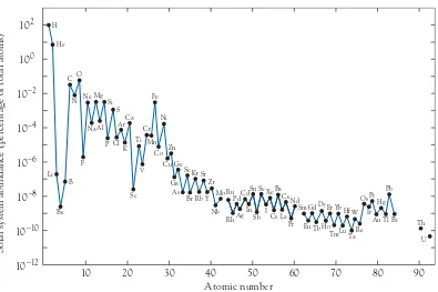
2.2 Existence of the Elements 23
2.3 Stability of the Elements and Their Isotopes 24
The Origin of the Shell Model of the Nucleus 26
2.4 Classifi cations of the Elements 27
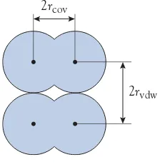
2.5 Periodic Properties: Atomic Radius 29
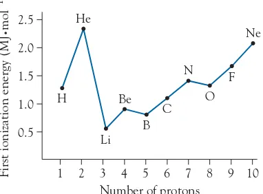
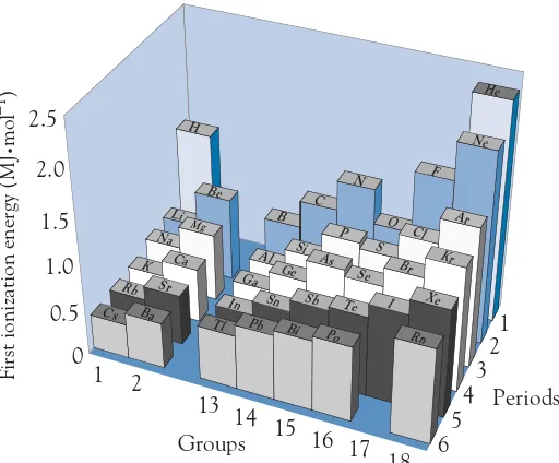
2.6 Periodic Properties: Ionization Energy 33
2.7 Periodic Properties: Electron Affi nity 35
Alkali Metal Anions 37
2.8 The Elements of Life 37
CHAPTER 3
Covalent Bonding
41
3.1 Models of Covalent Bonding 42
3.2 Introduction to Molecular Orbitals 43
3.3 Molecular Orbitals for Period 1
Diatomic Molecules 44
3.4 Molecular Orbitals for Period 2
Diatomic Molecules 46
3.5 Molecular Orbitals for Heteronuclear
Diatomic Molecules 50
3.6 A Brief Review of Lewis Structures 51
3.7 Partial Bond Order 53
3.8 Formal Charge 54
3.9 Valence-Shell Electron-Pair Repulsion Rules 54
3.10 The Valence-Bond Concept 59
3.11 Network Covalent Substances 61
3.12 Intermolecular Forces 63
The Origins of the Electronegativity Concept 65
3.13 Molecular Symmetry 66
3.13 Symmetry and Vibrational Spectroscopy 72
Transient Species—A New Direction for Inorganic
Chemistry 74
3.15 Covalent Bonding and the Periodic Table 78
CHAPTER 4
Metallic Bonding
81
4.1 Metallic Bonding 81
4.2 Bonding Models 82
4.3 Structure of Metals 84
4.4 Unit Cells 86
4.5 Alloys 87
Memory Metal: The Shape of Things to Come 88
4.6 Nanometal Particles 89
4.7 Magnetic Properties of Metals 90
CHAPTER 5
Ionic Bonding
93
5.1 The Ionic Model and the Size of Ions 93
5.2 Hydrated Salts 95
5.3 Polarization and Covalency 96
5.4 Ionic Crystal Structures 99
5.5 Crystal Structures Involving
Polyatomic Ions 105
5.6 The Bonding Continuum 106
Concrete: An Old Material with a New Future 109
CHAPTER 6
Inorganic Thermodynamics
113
6.1 Thermodynamics of the Formation
of Compounds 114
6.2 Formation of Ionic Compounds 120
6.3 The Born-Haber Cycle 122
6.4 Thermodynamics of the Solution
Process for Ionic Compounds 124
6.5 Formation of Covalent Compounds 127
The Hydrogen Economy 128
6.6 Thermodynamic versus Kinetic Factors 129
CHAPTER 7
Solvent Systems and Acid-Base
Behavior
137
7.1 Solvents 138
7.2 Brønsted-Lowry Acids 142
Antacids 144
7.3 Brønsted-Lowry Bases 147
Cyanide and Tropical Fish 148
7.4 Trends in Acid-Base Behavior 148
Superacids and Superbases 150
7.5 Acid-Base Reactions of Oxides 153
7.6 Lewis Theory 155
7.7 Pearson Hard-Soft Acid-Base Concepts 156
7.8 Applications of the HSAB Concept 158
7.9 Biological Aspects 161
CHAPTER 8
Oxidation and Reduction
167
8.1 Redox Terminology 167
8.2 Oxidation Number Rules 168
8.3 Determination of Oxidation Numbers
from Electronegativities 169
8.4 The Difference between Oxidation
Number and Formal Charge 171
8.5 Periodic Variations of Oxidation
Numbers 172
8.6 Redox Equations 173
Chemosynthesis: Redox Chemistry on the
Seafl oor 175
8.7 Quantitative Aspects of Half-Reactions 176
8.8 Electrode Potentials as Thermodynamic
Functions 177
8.9 Latimer (Reduction Potential) Diagrams 178
8.10 Frost (Oxidation State) Diagrams 180
8.11 Pourbaix Diagrams 182
8.12 Redox Synthesis 184
8.13 Biological Aspects 185
CHAPTER 9
Periodic Trends
191
9.1 Group Trends 192
9.2 Periodic Trends in Bonding 195
9.3 Isoelectronic Series in Covalent
Compounds 199
9.4 Trends in Acid-Base Properties 201
9.5 The (n) Group and (n !10) Group
Similarities 202
Chemical Topology 206
9.6 Isomorphism in Ionic Compounds 207
New Materials: Beyond the Limitations of
Geochemistry 209
9.7 Diagonal Relationships 210
Lithium and Mental Health 211
9.8 The “Knight’s Move” Relationship 212
9.9 The Early Actinoid Relationships 215
9.10 The Lanthanoid Relationships 216
9.11 “Combo” Elements 217
9.12 Biological Aspects 221
Thallium Poisoning: Two Case Histories 223
CHAPTER 10
Hydrogen
227
10.1 Isotopes of Hydrogen 228
10.2 Nuclear Magnetic Resonance 229
Isotopes in Chemistry 230
10.3 Properties of Hydrogen 231
Searching the Depths of Space for the
Trihydrogen Ion 233
10.4 Hydrides 233
10.5 Water and Hydrogen Bonding 237
Water: The New Wonder Solvent 238
vii
10.7 Biological Aspects of Hydrogen
Bonding 241
Is There Life Elsewhere in Our Solar System? 242
10.8 Element Reaction Flowchart 242
CHAPTER 11
The Group 1 Elements: The Alkali
Metals
245
11.1 Group Trends 246
11.2 Features of Alkali Metal Compounds 247
11.3 Solubility of Alkali Metal Salts 249
Mono Lake 250
11.9 Sodium Chloride 261
Salt Substitutes 261
11.10 Potassium Chloride 262
11.11 Sodium Carbonate 262
11.12 Sodium Hydrogen Carbonate 264
11.13 Ammonia Reaction 264
11.14 Ammonium Ion as a Pseudo–
Alkali-Metal Ion 265
11.15 Biological Aspects 265
11.16 Element Reaction Flowcharts 266
CHAPTER 12
The Group 2 Elements: The Alkaline
Earth Metals
271
12.1 Group Trends 271
12.2 Features of Alkaline Earth Metal
Compounds 272
12.3 Beryllium 275
12.4 Magnesium 276
12.5 Calcium and Barium 278
12.6 Oxides 279
12.7 Calcium Carbonate 280
How Was Dolomite Formed? 281
12.8 Cement 282
12.9 Calcium Chloride 283
Biomineralization: A New Interdisciplinary
“Frontier” 284
12.10 Calcium Sulfate 284
12.11 Calcium Carbide 285
12.12 Biological Aspects 286
12.15 Element Reaction Flowcharts 287
CHAPTER 13
The Group 13 Elements
291
13.1 Group Trends 292
13.2 Boron 293
13.3 Borides 294
Inorganic Fibers 295
13.4 Boranes 295
Boron Neutron Capture Therapy 298
13.5 Boron Halides 300
13.6 Aluminum 301
13.7 Aluminum Halides 306
13.8 Aluminum Potassium Sulfate 307
13.9 Spinels 308
13.10 Aluminides 309
13.11 Biological Aspects 309
13.12 Element Reaction Flowcharts 311
CHAPTER 14
The Group 14 Elements
315
14.1 Group Trends 316
14.2 Contrasts in the Chemistry of Carbon
and Silicon 316
14.3 Carbon 318
The Discovery of Buckminsterfullerene 322
14.4 Isotopes of Carbon 325
14.5 Carbides 326
Moissanite: The Diamond Substitute 327
14.6 Carbon Monoxide 328
14.7 Carbon Dioxide 330
Carbon Dioxide, Supercritical Fluid 332
14.8 Carbonates and Hydrogen Carbonates 333
14.9 Carbon Sulfi des 335
14.10 Carbon Halides 335
14.11 Methane 338
14.12 Cyanides 339
14.13 Silicon 339
14.14 Silicon Dioxide 341
14.15 Silicates 343
14.20 Tin and Lead Halides 353
14.21 Tetraethyllead 354
TEL: A Case History 355
14.22 Biological Aspects 356
14.23 Element Reaction Flowcharts 359
CHAPTER 15
The Group 15 Elements:
The Pnictogens
363
15.1 Group Trends 364
15.2 Contrasts in the Chemistry
of Nitrogen and Phosphorus 365
15.3 Overview of Nitrogen Chemistry 368
The First Dinitrogen Compound 369
15.4 Nitrogen 369
Propellants and Explosives 370
15.5 Nitrogen Hydrides 371
Haber and Scientifi c Morality 374
15.6 Nitrogen Ions 377
15.7 The Ammonium Ion 378
15.8 Nitrogen Oxides 379
15.9 Nitrogen Halides 384
15.10 Nitrous Acid and Nitrites 385
15.11 Nitric Acid and Nitrates 386
15.12 Overview of Phosphorus Chemistry 389
15.13 Phosphorus 390
Nauru, the World’s Richest Island 391
15.14 Phosphine 393
15.15 Phosphorus Oxides 393
15.16 Phosphorus Chlorides 394
15.17 Phosphorus Oxo-Acids and Phosphates 395
15.18 The Pnictides 399
15.19 Biological Aspects 399
Paul Erhlich and His “Magic Bullet” 401
15.29 Element Reaction Flowcharts 402
CHAPTER 16
The Group 16 Elements:
The Chalcogens
409
16.1 Group Trends 410
16.2 Contrasts in the Chemistry of
Oxygen and Sulfur 411
16.3 Oxygen 412
Oxygen Isotopes in Geology 412
16.4 Bonding in Covalent Oxygen
Compounds 418
16.5 Trends in Oxide Properties 419
16.6 Mixed-Metal Oxides 421
New Pigments through Perovskites 422
16.7 Water 422
16.8 Hydrogen Peroxide 424
16.9 Hydroxides 424
16.10 The Hydroxyl Radical 426
16.11 Overview of Sulfur Chemistry 426
16.12 Sulfur 427
Cosmochemistry: Io, the Sulfur-Rich Moon 428
16.13 Hydrogen Sulfi de 431
16.14 Sulfi des 432
Disulfi de Bonds and Hair 432
16.15 Sulfur Oxides 434
16.16 Sulfi tes 437
16.17 Sulfuric Acid 438
16.18 Sulfates and Hydrogen Sulfates 440
16.19 Other Oxy-Sulfur Anions 441
16.20 Sulfur Halides 443
16.21 Sulfur-Nitrogen Compounds 445
16.22 Selenium 445
16.23 Biological Aspects 446
16.24 Element Reaction Flowcharts 448
CHAPTER 17
The Group 17 Elements: The Halogens 453
17.1 Group Trends 454
17.2 Contrasts in the Chemistry of
Fluorine and Chlorine 455
17.3 Fluorine 458
The Fluoridation of Water 459
17.4 Hydrogen Fluoride and Hydrofl uoric Acid 460
ix
17.6 Chlorine 463
17.7 Hydrochloric Acid 464
17.8 Halides 465
17.9 Chlorine Oxides 469
17.10 Chlorine Oxyacids and Oxyanions 471
Swimming Pool Chemistry 473
The Discovery of the Perbromate Ion 474
17.11 Interhalogen Compounds and
Polyhalide Ions 475
17.12 Cyanide Ion as a Pseudo-halide Ion 477
17.13 Biological Aspects 478
17.14 Element Reaction Flowcharts 481
CHAPTER 18
The Group 18 Elements:
The Noble Gases
487
18.1 Group Trends 488
18.2 Unique Features of Helium 489
18.3 Uses of the Noble Gases 489
18.4 A Brief History of Noble Gas
Compounds 491
Is It Possible to Make Compounds of the
Early Noble Gases? 492
18.5 Xenon Fluorides 492
18.6 Xenon Oxides 494
18.7 Other Noble Gas Compounds 495
18.8 Biological Aspects 495
18.9 Element Reaction Flowchart 496
CHAPTER 19
Transition Metal Complexes
499
19.1 Transition Metals 499
19.2 Introduction to Transition Metal
Complexes 500
19.3 Stereochemistries 502
19.4 Isomerism in Transition Metal
Complexes 503
Platinum Complexes and Cancer Treatment 506
19.5 Naming Transition Metal Complexes 507
19.6 An Overview of Bonding Theories
of Transition Metal Compounds 510
19.7 Crystal Field Theory 511
19.8 Successes of Crystal Field Theory 517
The Earth and Crystal Structures 521
19.9 More on Electronic Spectra 521
19.10 Ligand Field Theory 523
19.11 Thermodynamic versus Kinetic Factors 525
19.12 Synthesis of Coordination Compounds 526
19.13 Coordination Complexes and the
HSAB Concept 527
19.14 Biological Aspects 529
CHAPTER 20
Properties of the 3d Transition
Metals
533
20.1 Overview of the 3d Transition Metals 534
20.2 Group 4: Titanium 536
20.3 Group 5: Vanadium 537
20.4 Group 6: Chromium 538
20.5 Group 7: Manganese 544
Mining the Seafl oor 545
20.6 Group 8: Iron 549
20.7 Group 9: Cobalt 558
20.8 Group 10: Nickel 562
20.9 Group 11: Copper 563
20.10 Biological Aspects 569
20.11 Element Reaction Flowcharts 572
CHAPTER 21
Properties of the 4d and 5d
Transition Metals
579
21.1 Comparison of the Transition Metals 580
21.2 Features of the Heavy
Transition Metals 581
21.3 Group 4: Zirconium and Hafnium 584
21.4 Group 5: Niobium and Tantalum 585
21.5 Group 6: Molybdenum and Tungsten 586
21.6 Group 7: Technetium and Rhenium 587
Technetium: The Most Important
Radiopharmaceutical 588
21.7 The Platinum Group Metals 589
21.8 Group 8: Ruthenium and Osmium 590
21.9 Group 9: Rhodium and Iridium 591
21.10 Group 10: Palladium and Platinum 591
21.11 Group 11: Silver and Gold 591
21.12 Biological Aspects 594
CHAPTER 22
The Group 12 Elements
599
22.1 Group Trends 600
22.2 Zinc and Cadmium 600
22.3 Mercury 603
22.4 Biological Aspects 605
Mercury Amalgam in Teeth 607
22.5 Element Reaction Flowchart 608
CHAPTER 23
Organometallic Chemistry
611
23.1 Introduction to Organometallic
Compounds 612
23.2 Naming Organometallic Compounds 612
23.3 Counting Electrons 613
23.4 Solvents for Organometallic Chemistry 614
23.5 Main Group Organometallic
Compounds 615
Grignard Reagents 618
The Death of Karen Wetterhahn 623
23.6 Organometallic Compounds of the
Transition Metals 623
23.7 Transition Metal Carbonyls 625
23.8 Synthesis and Properties of Simple
Metal Carbonyls 630
23.9 Reactions of Transition Metal Carbonyls 632
23.10 Other Carbonyl Compounds 633
23.11 Complexes with Phosphine Ligands 634
23.12 Complexes with Alkyl, Alkene, and
Alkyne Ligands 635
Vitamin B12—A Naturally Occurring
Organometallic Compound 638
23.13 Complexes with Allyl and 1,3-Butadiene
Ligands 639
23.14 Metallocenes 640
23.15 Complexes with "6-Arene Ligands 642
23.16 Complexes with Cycloheptatriene and
Cyclooctatetraene Ligands 643
23.17 Fluxionality 643
23.18 Organometallic Compounds in
Industrial Catalysis 644
CHAPTER 24
ON THE WEB www.whfreeman.com/descriptive5e
The Rare Earth and Actinoid
Elements
651w
24.1 The Group 3 Elements 653w
24.2 The Lanthanoids 653w
Superconductivity 655w
23.3 The Actinoids 656w
24.4 Uranium 659w
A Natural Fission Reactor 661w
24.5 The Postactinoid Elements 662w
APPENDICES
Appendix 1 Thermodynamic Properties of Some Selected Inorganic
Compounds A-1
Appendix 2 Charge Densities of Selected
Ions A-13
Appendix 3 Selected Bond Energies A-16
Appendix 4 Ionization Energies of Selected
Metals A-18
Appendix 5 Electron Affi nities of Selected
Nonmetals A-20
Appendix 6 Selected Lattice Energies A-21
Appendix 7 Selected Hydration Enthalpies A-22
Appendix 8 Selected Ionic Radii A-23
ON THE WEB www.whfreeman.com/descriptive5e Appendix 9 Standard Half-Cell Electrode
Potentials of Selected
Elements A-25w
ON THE WEB www.whfreeman.com/descriptive5e Appendix 10 Electron Confi guration
of the Elements A-35w
What Is Descriptive Inorganic Chemistry?
D
escriptive inorganic chemistry was traditionally concerned with the prop-erties of the elements and their compounds. Now, in the renaissance of the subject, with the synthesis of new and novel materials, the properties are being linked with explanations for the formulas and structures of compounds together with an understanding of the chemical reactions they undergo. In addition, we are no longer looking at inorganic chemistry as an isolated subject but as a part of essential scientifi c knowledge with applications throughout science and our lives. Because of a need for greater contextualization, we have added more features and more applications.In many colleges and universities, descriptive inorganic chemistry is offered as a sophomore or junior course. In this way, students come to know something of the fundamental properties of important and interesting elements and their compounds. Such knowledge is important for careers not only in pure or applied chemistry but also in pharmacy, medicine, geology, and environmental science. This course can then be followed by a junior or senior course that focuses on the theoretical principles and the use of spectroscopy to a greater depth than is covered in a descriptive text. In fact, the theoretical course builds nicely on the descriptive background. Without the descriptive grounding, however, the theory becomes sterile, uninteresting, and irrelevant.
Education has often been a case of the “swinging pendulum,” and this has been true of inorganic chemistry. Up until the 1960s, it was very much pure descriptive, requiring exclusively memorization. In the 1970s and 1980s, upper-level texts focused exclusively on the theoretical principles. Now it is ap-parent that descriptive is very important—not the traditional memorization of facts but the linking of facts, where possible, to underlying principles. Students need to have modern descriptive inorganic chemistry as part of their educa-tion. Thus, we must ensure that chemists are aware of the “new descriptive inorganic chemistry.”
Preface
Inorganic chemistry goes beyond academic interest: it is an
im-portant part of our lives.
I
norganic chemistry is interesting—more than that—it is exciting! So much of our twenty-fi rst-century science and technology rely on natural and syn-thetic materials, often inorganic compounds, many of which are new and novel. Inorganic chemistry is ubiquitous in our daily lives: household products, some pharmaceuticals, our transportation—both the vehicles themselves and the synthesis of the fuels—battery technology, and medical treatments. There is the industrial aspect, the production of all the chemicals required to drive our economy, everything from steel to sulfuric acid to glass and cement. Environ-mental chemistry is largely a question of the inorganic chemistry of the atmo-sphere, water, and soil. Finally, there are the profound issues of the inorganic chemistry of our planet, the solar system, and the universe.This textbook is designed to focus on the properties of selected interesting, important, and unusual elements and compounds. However, to understand inorganic chemistry, it is crucial to tie this knowledge to the underlying chemi-cal principles and hence provide explanations for the existence and behavior of compounds. For this reason, almost half the chapters survey the relevant concepts of atomic theory, bonding, intermolecular forces, thermodynamics, acid-base behavior, and reduction-oxidation properties as a prelude to, and preparation for, the descriptive material.
For this fi fth edition, the greatest change has been the expansion of coverage of the 4d and 5d transition metals to a whole chapter.
The heavier transition metals have unique trends and patterns, and the new chapter highlights these. Having an additional chapter on transition met-als met-also better balances the coverage between the main group elements and the transition elements.
Also, the fi fth edition has a second color. With the addition of a second color, fi gures are much easier to understand, and tables and text are easier to read.
On a chapter-by-chapter basis, the signifi cant improvements are as follows:
Chapter 1: The Electronic Structure of the Atom: A Review
The Introduction and Section 1.3, The Polyelectronic Atom, have been revised. Chapter 3: Covalent Bonding
Section 3.11, Network Covalent Substances, has a new subsection: Amorphous Silicon.
Chapter 4: Metallic Bonding
Section 4.6, Nanometal Particles, was added.
Section 4.7, Magnetic Properties of Metals, was added.
Chapter 5: Ionic Bonding
Section 5.3, Polarization and Covalency, has a new subsection: The Ionic-Covalent Boundary.
Section 5.4, Ionic Crystal Structures, has a new subsection: Quantum Dots. Chapter 9: Periodic Trends
Section 9.3, Isoelectronic Series in Covalent Compounds, has been revised and improved.
Section 9.8, The “Knight’s Move” Relationship, has been revised and improved. Chapter 10: Hydrogen
Section 10.4, Hydrides, has a revised and expanded subsection: Ionic Hydrides. Chapter 11: The Group 1 Elements
Section 11.14, Ammonium Ion as a Pseudo–Alkali-Metal Ion, moved from Chapter 9.
Chapter 13: The Group 13 Elements Section 13.10, Aluminides, was added. Chapter 14: The Group 14 Elements
Section 14.2, Contrasts in the Chemistry of Carbon and Silicon, was added. Section 14.3, Carbon, has a new subsection: Graphene.
Section 14.7, Carbon Dioxide, has a new subsection: Carbonia. Chapter 15: The Group 15 Elements
Section 15.2, Contrasts in the Chemistry of Nitrogen and Phosphorus, was added.
Section 15.18, The Pnictides, was added. Chapter 16: The Group 16 Elements
Section 16.2, Contrasts in the Chemistry of Oxygen and Sulfur, was added. Section 16.14, Sulfi des, has a new subsection: Disulfi des.
Chapter 17: The Group 17 Elements
Section 17.2, Contrasts in the Chemistry of Fluorine and Chlorine, was added. Section 17.12, Cyanide Ion as a Pseudo-halide Ion, moved from Chapter 9. Chapter 18: The Group 18 Elements
Section 18.7, Other Noble Gas Compounds, was added. Chapter 19: Transition Metal Complexes
Section 19.10, Ligand Field Theory, was added. Chapter 20: Properties of the 3d Transition Metals
Section 20.1, Overview of the 3d Transition Metals, was added. Chapter 21: Properties of the 4d and 5d Transition Metals NEW CHAPTERadded (for details, see the previous page). Chapter 24: The Rare Earth and Actinoid Elements
xv
ALSO Video Clips
Descriptive inorganic chemistry by defi nition is visual, so what better way to appreciate a chemical reaction than to make it visual? We now have a series of at least 60 Web-based video clips to bring some of the reactions to life. The text has a margin icon to indicate where a reaction is illustrated.
Text Figures and Tables
All the illustrations and tables in the book are available as .jpg fi les for inclusion in PowerPoint presentations on the instructor side of the Web site at www.whfreeman.com/descriptive5e.
Additional Resources
A list of relevant SCIENTIFIC AMERICANarticles is found on the text Web site at www.whfreeman.com/descriptive5e. The text has a margin icon to indicate where a Scientifi c American article is available.
Supplements
The Student Solutions Manual, ISBN: 1-4292-2434-7 contains the worked solutions to all the odd-numbered end-of-chapter problems.
The Companion Web Sitewww.whfreeman.com/descriptive5e
Contains the following student-friendly materials: Chapter 24: The Rare Earth and Actinoid Elements, Appendices, Lab Experiments, Tables, and over 50 useful videos of elements and metals in reactions and oxidations.
Instructor’s Resource CD-ROM, ISBN: 1-4292-2428-2
Includes PowerPoint and videos as well as all text art and solutions to all prob-lems in the book.
This textbook was written to pass on to another generation our fascination with descriptive inorganic chemistry. Thus, the comments of readers, both stu-dents and instructors, will be sincerely appreciated. Any suggestions for added or updated additional readings are also welcome. Our current e-mail addresses [email protected] and [email protected].
Acknowledgments
M
any thanks must go to the team at W. H. Freeman and Company who have contributed their talents to the fi ve editions of this book. We offer our sincere gratitude to the editors of the fi fth edition, Jessica Fiorillo, Kathryn Treadway, and Mary Louise Byrd; of the fourth edition, Jessica Fiorillo, Jenness Crawford, and Mary Louise Byrd; of the third edition, Jessica Fiorillo and Guy Copes; of the second edition, Michelle Julet and Mary Louise Byrd; and a special thanks to Deborah Allen, who bravely commissioned the fi rst edition of the text. Each one of our fabulous editors has been a source of encouragement, support, and helpfulness.We wish to acknowledge the following reviewers of this edition, whose criticisms and comments were much appreciated: Theodore Betley at Harvard University; Dean Campbell at Bradley University; Maria Contel at Brooklyn College (CUNY); Gerry Davidson at St. Francis College; Maria Derosa at Carleton University; Stan Duraj at Cleveland State University; Dmitri Giarkios at Nova Southeastern University; Michael Jensen at Ohio University–Main Campus; David Marx at the University of Scranton; Joshua Moore at Tennessee State University–Nashville; Stacy O’Reilly at Butler University; William Pen-nington at Clemson University; Daniel Rabinovich at the University of North Carolina at Charlotte; Hal Rogers at California State University–Fullerton; Thomas Schmedake at the University of North Carolina at Charlotte; Bradley Smucker at Austin College; Sabrina Sobel at Hofstra University; Ronald Strange at Fairleigh Dickinson University–Madison; Mark Walters at New York University; Yixuan Wang at Albany State University; and Juchao Yan at Eastern New Mexico University; together with prereviewers: Londa Borer at California State University–Sacramento; Joe Fritsch at Pepperdine Univer-sity; Rebecca Roesner at Illinois Wesleyan University, and Carmen Works at Sonoma College.
We acknowledge with thanks the contributions of the reviewers of the fourth edition: Rachel Narehood Austin at Bates College; Leo A. Bares at the University of North Carolina—Asheville; Karen S. Brewer at Hamilton College; Robert M. Burns at Alma College; Do Chang at Averett University; Georges Dénès at Concordia University; Daniel R. Derringer at Hollins University; Carl P. Fictorie at Dordt College; Margaret Kastner at Bucknell University; Michael Laing at the University of Natal, Durban; Richard H. Langley at Stephen F. Austin State University; Mark R. McClure at the University of North Carolina at Pembroke; Louis Mercier at Laurentian University; G. Merga at Andrews University; Stacy O’Reilly at Butler University; Larry D. Pedersen at College Misercordia; Robert D. Pike at the College of William and Mary; William Quintana at New Mexico State University; David F. Rieck at Salisbury University; John Selegue at the University of Kentucky; Melissa M. Strait at Alma College; Daniel J. Williams at Kennesaw State University; Juchao Yan at Eastern New Mexico University; and Arden P. Zipp at the State University of New York at Cortland.
And the contributions of the reviewers of the third edition: François Caron at Laurentian University; Thomas D. Getman at Northern Michigan Univer-sity; Janet R. Morrow at the State University of New York at Buffalo; Robert D. Pike at the College of William and Mary; Michael B. Wells at Cambell Uni-versity; and particularly Joe Takats of the University of Alberta for his compre-hensive critique of the second edition.
And the contributions of the reviewers of the second edition: F. C. Hentz at North Carolina State University; Michael D. Johnson at New Mexico State University; Richard B. Kaner at the University of California, Los Angeles; Richard H. Langley at Stephen F. Austin State University; James M. Mayer at the University of Washington; Jon Melton at Messiah College; Joseph S. Merola at Virginia Technical Institute; David Phillips at Wabash College; John R. Pladziewicz at the University of Wisconsin, Eau Claire; Daniel Rabinovich at the University of North Carolina at Charlotte; David F. Reich at Salisbury State University; Todd K. Trout at Mercyhurst College; Steve Watton at the Virginia Commonwealth University; and John S. Wood at the University of Massachusetts, Amherst.
Likewise, the reviewers of the fi rst edition: E. Joseph Billo at Boston Col-lege; David Finster at Wittenberg University; Stephen J. Hawkes at Oregon State University; Martin Hocking at the University of Victoria; Vake Marganian at Bridgewater State College; Edward Mottel at the Rose-Hulman Institute of Technology; and Alex Whitla at Mount Allison University.
As a personal acknowledgment, Geoff Rayner-Canham wishes to especial-ly thank three teachers and mentors who had a major infl uence on his career: Briant Bourne, Harvey Grammar School; Margaret Goodgame, Imperial Col-lege, London University; and Derek Sutton, Simon Fraser University. And he expresses his eternal gratitude to his spouse, Marelene, for her support and encouragement.
Dedication
C
hemistry is a human endeavor. New discoveries are the result of the work of enthusiastic people and groups of people who want to explore the molecular world. We hope that you, the reader, will come to share our own fascination with inorganic chemistry. We have chosen to dedicate this book to two scientists who, for very different reasons, never did receive the ultimate accolade of a Nobel Prize.Henry Moseley (1887–1915)
Although Mendeleev is identifi ed as the discoverer of the peri-odic table, his version was based on an increase in atomic mass. In some cases, the order of elements had to be reversed to match properties with location. It was a British scientist, Henry Moseley, who put the periodic table on a much fi rmer footing by discov-ering that, on bombardment with electrons, each element emit-ted X-rays of characteristic wavelengths. The wavelengths fi temit-ted a formula related by an integer number unique to each element. We know that number to be the number of protons. With the es-tablishment of the atomic number of an element, chemists at last knew the fundamental organization of the table. Sadly, Moseley was killed at the battle of Gallipoli in World War I. Thus, one of the brightest scientifi c talents of the twentieth century died at the
age of 27. The famous American scientist Robert Milliken commented: “Had the European War had no other result than the snuffi ng out of this young life, that alone would make it one of the most hideous and most irreparable crimes in history.” Unfortunately, Nobel Prizes are only awarded to living scientists. In 1924, the discovery of element 43 was claimed, and it was named mose-leyum; however, the claim was disproved by the very method that Moseley had pioneered.
Lise Meitner (1878–1968)
In the 1930s, scientists were bombarding atoms of heavy elements such as uranium with subatomic particles to try to make new ele-ments and extend the periodic table. Austrian scientist Lise Meit-ner had shared leadership with Otto Hahn of the German research team working on the synthesis of new elements; the team thought they had discovered nine new elements. Shortly after the claimed discovery, Meitner was forced to fl ee Germany because of her Jewish ancestry, and she settled in Sweden. Hahn reported to her that one of the new elements behaved chemically just like barium. During a famous “walk in the snow” with her nephew, physicist Otto Frisch, Meitner realized that an atomic nucleus could break in two just like a drop of water. No wonder the element formed behaved like barium: it was barium! Thus was born the concept of nuclear fi ssion. She informed Hahn of her proposal. When Hahn wrote the research paper on the work, he barely mentioned the vital contribution of Meitner and Frisch. As a result, Hahn and his colleague Fritz Strassmann received the Nobel Prize. Meitner’s fl ash of genius was ignored. Only recently has Meitner received the acclaim she deserved by the naming of an element after her, element 109, meitnerium.
Additional reading
Heibron, J. L. H. G. J. Moseley. University of California Press, Berkeley, 1974. Rayner-Canham, M. F., and G. W. Rayner-Canham. Women in Chemistry: Their Changing Roles from Alchemical Times to the Mid-Twentieth Century. Chemical Heritage Foundation, Philadelphia, 1998.
Sime, R. L. Lise Meitner: A Life in Physics. University of California Press, Berkeley, 1996.
I
saac Newton was the original model for the absentminded professor. Supposedly, he always timed the boiled egg he ate at breakfast; one morning, his maid found him standing by the pot of boiling water, hold-ing an egg in his hand and gazhold-ing intently at the watch in the bottom of the pot! Nevertheless, it was Newton who initiated the study of the electronic structure of the atom in about 1700, when he noticed that the passage of sunlight through a prism produced a continuous visible spectrum. Much later, in 1860, Robert Bunsen (of burner fame) inves-tigated the light emissions from fl ames and gases. Bunsen observed that the emission spectra, rather than being continuous, were series of colored lines (line spectra).The proposal that electrons existed in concentric shells had its origin in the research of two overlooked pioneers: Johann Jakob Balmer, a Swiss mathematician, and Johannes Robert Rydberg, a Swedish physicist. After an undistinguished career in mathematics, in 1885, at the age of 60, Balmer studied the visible emission lines of the hydrogen atom and found that there was a mathematical relationship between the wave-lengths. Following from Balmer’s work, in 1888, Rydberg deduced a more general relationship:
1
l5RHa
1
n2f
2 1
n2i b
wherel is the wavelength of the emission line, RH is a constant, later
known as the Rydberg constant, and nf and ni are integers. For the
visible lines seen by Balmer and Rydberg, nf had a value of 2. The
Rydberg formula received further support in 1906, when Theodore Lyman found a series of lines in the far-ultraviolet spectrum of hydrogen,
1.1 The Schrödinger Wave Equation and Its Signifi cance
Atomic Absorption Spectroscopy
1.2 Shapes of the Atomic Orbitals
1.3 The Polyelectronic Atom
1.4 Ion Electron Confi gurations
1.5 Magnetic Properties of Atoms
1.6 Medicinal Inorganic Chemistry: An Introduction
The Electronic Structure
of the Atom: A Review
C HA P TE R
1
1
To understand the behavior of inorganic compounds, we need to study
the nature of chemical bonding. Bonding, in turn, relates to the behavior
of electrons in the constituent atoms. Our study of inorganic chemistry,
therefore, starts with a review of the models of the atom and a survey of
the probability model’s applications to the electron confi gurations of atoms
corresponding to the Rydberg formula with nf51. Then in 1908, Friedrich
Paschen discovered a series of far-infrared hydrogen lines, fi tting the equation with nf53.
In 1913, Niels Bohr, a Danish physicist, became aware of Balmer’s and Rydberg’s experimental work and of the Rydberg formula. At that time, he was trying to combine Ernest Rutherford’s planetary model for electrons in an atom with Max Planck’s quantum theory of energy exchanges. Bohr contended that an electron orbiting an atomic nucleus could only do so at certain fi xed distances and that whenever the electron moved from a higher to a lower orbit, the atom emitted characteristic electromagnetic radiation.
Rydberg had deduced his equation from experimental observations of atomic hydrogen emission spectra. Bohr was able to derive the same equation from quantum theory, showing that his theoretical work meshed with reality. From this result, the Rutherford-Bohr model of the atom of concentric elec-tron “shells” was devised, mirroring the recurring patterns in the periodic table of the elements (Figure 1.1). Thus the whole concept of electron energy levels can be traced back to Rydberg. In recognition of Rydberg’s contribution, excited atoms with very high values of the principal quantum number, n, are called Rydberg atoms.
However, the Rutherford-Bohr model had a number of fl aws. For example, the spectra of multi-electron atoms had far more lines than the simple Bohr model predicted. Nor could the model explain the splitting of the spectral lines in a magnetic fi eld (a phenomenon known as the Zeeman effect). Within a short time, a radically different model, the quantum mechanical model, was proposed to account for these observations.
n#3
n#2 n#1
!Ze $E#hv
FIGURE 1.1 The Rutherford-Bohr electron-shell model of the atom, showing the n51, 2, and 3 energy levels.
A
glowing body, such as the Sun, is expected to emit a continuous spectrum of electromagnetic radiation. However, in the early nineteenth century, a German sci-entist, Josef von Fraunhofer, noticed that the visible spec-trum from the Sun actually contained a number of dark bands. Later investigators realized that the bands were the result of the absorption of particular wavelengths by cooler atoms in the “atmosphere” above the surface of the Sun. The electrons of these atoms were in the ground state, and they were absorbing radiation at wavelengths corresponding to the energies needed to excite them to higher energy states. A study of these “negative” spectra led to the discovery of helium. Such spectral studies are still of great importance in cosmochemistry—the study of the chemical composition of stars.In 1955, two groups of scientists, one in Australia and the other in Holland, fi nally realized that the absorption method could be used to detect the presence of elements
at very low concentrations. Each element has a particu-lar absorption spectrum corresponding to the various separations of (differences between) the energy levels in its atoms. When light from an atomic emission source is passed through a vaporized sample of an element, the particular wavelengths corresponding to the various en-ergy separations will be absorbed. We fi nd that the higher the concentration of the atoms, the greater the proportion of the light that will be absorbed. This linear relationship between light absorption and concentration is known as
Beer’s law. The sensitivity of this method is extremely high, and concentrations of parts per million are easy to determine; some elements can be detected at the parts per billion level. Atomic absorption spectroscopy has now become a routine analytical tool in chemistry, metal-lurgy, geology, medicine, forensic science, and many other fi elds of science—and it simply requires the movement of electrons from one energy level to another.
3
1.1
The Schrödinger Wave Equation and Its Signifi cance
The more sophisticated quantum mechanical model of atomic structure was derived from the work of Louis de Broglie. De Broglie showed that, just as elec-tromagnetic waves could be treated as streams of particles (photons), moving particles could exhibit wavelike properties. Thus, it was equally valid to picture electrons either as particles or as waves. Using this wave-particle duality, Erwin Schrödinger developed a partial differential equation to represent the behavior of an electron around an atomic nucleus. One form of this equation, given here for a one-electron atom, shows the relationship between the wave function of the electron, C, and E and V, the total and potential energies of the system, re-spectively. The second differential terms relate to the wave function along each of the Cartesian coordinates x,y, and z, while m is the mass of an electron, and
h is Planck’s constant.
02° 0x2 1
02° 0y2 1
02° 0z2 1
8p2m
h2 1E2V2° 50
The derivation of this equation and the method of solving it are in the realm of physics and physical chemistry, but the solution itself is of great importance to inorganic chemists. We should always keep in mind, however, that the wave equation is simply a mathematical formula. We attach meanings to the solution simply because most people need concrete images to think about subatomic phenomena. The conceptual models that we create in our macroscopic world cannot hope to reproduce the subatomic reality.
It was contended that the real meaning of the equation could be found from the square of the wave function, C2, which represents the probability of fi nding the electron at any point in the region surrounding the nucleus. There are a number of solutions to a wave equation. Each solution describes a different orbital and, hence, a different probability distribution for an elec-tron in that orbital. Each of these orbitals is uniquely defi ned by a set of three integers: n,l, and ml. Like the integers in the Bohr model, these integers are
also called quantum numbers.
In addition to the three quantum numbers derived from the original theory, a fourth quantum number had to be defi ned to explain the results of an experi-ment in 1922. In this experiexperi-ment, Otto Stern and Walther Gerlach found that passing a beam of silver atoms through a magnetic fi eld caused about half the atoms to be defl ected in one direction and the other half in the opposite direc-tion. Other investigators proposed that the observation was the result of two different electronic spin orientations. The atoms possessing an electron with one spin were defl ected one way, and the atoms whose electron had the oppo-site spin were defl ected in the oppooppo-site direction. This spin quantum number was assigned the symbol ms.
The possible values of the quantum numbers are defi ned as follows:
n, the principal quantum number, can have all positive integer values from 1 to q.
l, the angular momentum quantum number, can have all integer values fromn21 to 0.
ml, the magnetic quantum number, can have all integer values from 1l
through 0 to 2l.
ms, the spin quantum number, can have values of 112 and 212.
When the value of the principal quantum number is 1, there is only one possible set of quantum numbers n,l, and ml (1, 0, 0), whereas for a principal
quantum number of 2, there are four sets of quantum numbers (2, 0, 0; 2, 1, –1; 2, 1, 0; 2, 1, 11). This situation is shown diagrammatically in Figure 1.2. To identify the electron orbital that corresponds to each set of quantum numbers, we use the value of the principal quantum number n, followed by a letter for the angular momentum quantum number l. Thus, when n51, there is only the 1s orbital.
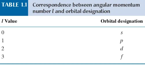
When n52, there is one 2s orbital and three 2p orbitals (corresponding to the ml values of 11, 0, and –1). The letters s,p,d, and f are derived from
categories of the spectral lines: sharp, principal, diffuse, and fundamental. The correspondences are shown in Table 1.1.
When the principal quantum number n53, there are nine sets of quantum numbers (Figure 1.3). These sets correspond to one 3s, three 3p, and fi ve 3d
orbitals. A similar diagram for the principal quantum number n54 would show 16 sets of quantum numbers, corresponding to one 4s, three 4p, fi ve 4d,
FIGURE 1.2 The possible sets of quantum numbers for n5 1 andn5 2.
n
l
ml
1s 2s 2p
%1 0 !1 0
0 1
1
0
0
2
TABLE 1.1 Correspondence between angular momentum numberl and orbital designation
l Value Orbital designation
0 s
1 p
2 d
1.2
Shapes of the Atomic Orbitals
Representing the solutions to a wave equation on paper is not an easy task. In fact, we would need four-dimensional graph paper (if it existed) to display the complete solution for each orbital. As a realistic alternative, we break the wave equation into two parts: a radial part and an angular part.
Each of the three quantum numbers derived from the wave equation rep-resents a different aspect of the orbital:
The principal quantum number n indicates the size of the orbital. The angular momentum quantum number l represents the shape of the orbital.
The magnetic quantum number ml represents the spatial direction of the
orbital.
The spin quantum number ms has little physical meaning; it merely allows
two electrons to occupy the same orbital.
It is the value of the principal quantum number and, to a lesser extent the angular momentum quantum number, which determines the energy of the electron. Although the electron may not literally be spinning, it behaves as if it was, and it has the magnetic properties expected for a spinning particle.
An orbital diagram is used to indicate the probability of fi nding an electron at any point in space. We defi ne a location where an electron is most probably
TABLE 1.2 Correspondence between angular momentum numberl and number of orbitals
l Value Number of orbitals
0 1
1 3
2 5
3 7
FIGURE 1.3 The possible sets of quantum numbers for n53.
n
l
ml
0 1
3
0 !1
%1 %2 %1 !1 !2
0 0
2
3s 3p 3d
and seven 4f orbitals (Table 1.2). Theoretically, we can go on and on, but as we will see, the f orbitals represent the limit of orbital types among the elements of the periodic table for atoms in their electronic ground states.
found as an area of high electron density. Conversely, locations with a low prob-ability are called areas of low electron density.
Thes Orbitals
The s orbitals are spherically symmetric about the atomic nucleus. As the prin-cipal quantum number increases, the electron tends to be found farther from the nucleus. To express this idea in a different way, we say that, as the principal quantum number increases, the orbital becomes more diffuse. A unique fea-ture of electron behavior in an s orbital is that there is a fi nite probability of fi nding the electron close to, and even within, the nucleus. This penetration by
s orbital electrons plays a role in atomic radii (see Chapter 2) and as a means of studying nuclear structure.
Same-scale representations of the shapes (angular functions) of the 1s and 2s orbitals of an atom are compared in Figure 1.4. The volume of a 2s orbital is about four times greater than that of a 1s orbital. In both cases, the tiny nucleus is located at the center of the spheres. These spheres represent the region in which there is a 99 percent probability of fi nding an electron. The total prob-ability cannot be represented, for the probprob-ability of fi nding an electron drops to zero only at an infi nite distance from the nucleus.
The probability of fi nding the electron within an orbital will always be posi-tive (since the probability is derived from the square of the wave function and squaring a negative makes a positive). However, when we discuss the bonding of atoms, we fi nd that the sign related to the original wave function has impor-tance. For this reason, it is conventional to superimpose the sign of the wave function on the representation of each atomic orbital. For an s orbital, the sign is positive.
In addition to the considerable difference in size between the 1s and the 2s
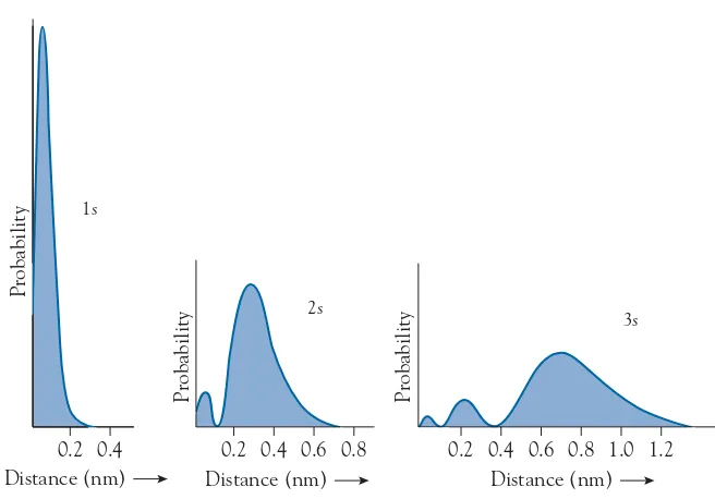
orbitals, the 2s orbital has, at a certain distance from the nucleus, a spherical surface on which the electron density is zero. A surface on which the probabil-ity of fi nding an electron is zero is called a nodal surface. When the principal quantum number increases by 1, the number of nodal surfaces also increases by 1. We can visualize nodal surfaces more clearly by plotting a graph of the ra-dial density distribution function as a function of distance from the nucleus for any direction. Figure 1.5 shows plots for the 1s, 2s, and 3s orbitals. These plots show that the electron tends to be farther from the nucleus as the principal quantum number increases. The areas under all three curves are the same.
7
Electrons in an s orbital are different from those in p,d, or f orbitals in two signifi cant ways. First, only the s orbital has an electron density that varies in the same way in every direction out from the atomic nucleus. Second, there is a fi nite probability that an electron in an s orbital is at the nucleus of the atom. Every other orbital has a node at the nucleus.
Thep Orbitals
Unlike the s orbitals, the p orbitals consist of two separate volumes of space (lobes), with the nucleus located between the two lobes. Because there are threep orbitals, we assign each orbital a direction according to Cartesian co-ordinates: we have px,py, and pz. Figure 1.6 shows representations of the three
2p orbitals. At right angles to the axis of higher probability, there is a nodal plane through the nucleus. For example, the 2pz orbital has a nodal surface in
thexy plane. In terms of wave function sign, one lobe is positive and the other negative.
FIGURE 1.5 The variation of the radial density distribution function with distance from the nucleus for electrons in the 1s, 2s, and 3s orbitals of a hydrogen atom.
2s
Distance (nm) 0.2 0.4 0.6 0.8 0.2 0.4 0.6 0.8 1.0 1.2 Distance (nm)
Probability
1s
0.2 0.4 Distance (nm)
Probability Probability
3s
1.2 Shapes of the Atomic Orbitals
FIGURE 1.6 Representations of the shapes of the 2px, 2py, and 2pz
If we compare graphs of electron density as a function of atomic radius for the 2s orbital and a 2p orbital (the latter plotted along the axis of higher prob-ability), we fi nd that the 2s orbital has a much greater electron density close to the nucleus than does the 2p orbital (Figure 1.7). Conversely, the second maximum of the 2s orbital is farther out than the single maximum of the 2p
orbital. However, the mean distance of maximum probability is the same for both orbitals.
Like the s orbitals, the p orbitals develop additional nodal surfaces within the orbital structure as the principal quantum number increases. Thus, a 3p
orbital does not look exactly like a 2p orbital since it has an additional nodal surface. However, the detailed differences in orbital shapes for a particular angular momentum quantum number are of little relevance in the context of basic inorganic chemistry.
Thed Orbitals
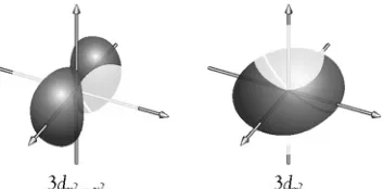
The fi ve d orbitals have more complex shapes. Three of them are located between the Cartesian axes, and the other two are oriented along the axes. In all cases, the nucleus is located at the intersection of the axes. Three orbitals each have four lobes that are located between pairs of axes (Figure 1.8). These orbitals are identifi ed as dxy, dxz, anddyz. The other two d orbitals, dz2 and dx22y2, are shown
in Figure 1.9. The dz2 orbital looks somewhat similar to a pz orbital (see Figure 1.6),
except that it has an additional doughnut-shaped ring of high electron density in the xy plane. The dx22y2 orbital is identical to the dxy orbital but has been
rotated through 458.
FIGURE 1.7 The variation of the radial density distribution function with distance from the nucleus for electrons in the 2s and 2p orbitals of a hydrogen atom.
2s
Distance (nm)
Probability
0.2 0.4 0.6 0.8
2p
Distance (nm)
Probability
0.2 0.4 0.6 0.8
9
Thef Orbitals
The f orbitals are even more complex than the d orbitals. There are seven
f orbitals, four of which have eight lobes. The other three look like the dz2
orbital but have two doughnut-shaped rings instead of one. These orbitals are rarely involved in bonding, so we do not need to consider them in any detail.
1.3
The Polyelectronic Atom
In our model of the polyelectronic atom, the electrons are distributed among the orbitals of the atom according to the Aufbau (building-up) principle. This simple idea proposes that, when the electrons of an atom are all in the ground state, they occupy the orbitals of lowest energy, thereby minimizing the atom’s total electronic energy. Thus, the confi guration of an atom can be described simply by adding electrons one by one until the total number required for the element has been reached.
Before starting to construct electron confi gurations, we need to take into account a second rule: the Pauli exclusion principle. According to this rule, no two electrons in an atom may possess identical sets of the four quantum num-bers. Thus, there can be only one orbital of each three-quantum-number set per atom and each orbital can hold only two electrons, one with ms5 112 and
the other with ms5 212.
Filling the s Orbitals
The simplest confi guration is that of the hydrogen atom. According to the Aufbau principle, the single electron will be located in the 1s orbital. This con-fi guration is the ground state of the hydrogen atom. Adding energy would raise the electron to one of the many higher energy states. These confi gurations are referred to as excited states. In the diagram of the ground state of the hydro-gen atom (Figure 1.10), a half-headed arrow is used to indicate the direction of electron spin. The electron confi guration is written as 1s1, with the superscript 1 indicating the number of electrons in that orbital.
1.3 The Polyelectronic Atom
1s
FIGURE 1.10 Electron
confi guration of a hydrogen atom.
With a two-electron atom (helium), there is a choice: the second electron could go in the 1s orbital (Figure 1.11a) or the next higher energy orbital, the 2s
orbital (Figure 1.11b). Although it might seem obvious that the second electron would enter the 1s orbital, it is not so simple. If the second electron entered the 1s orbital, it would be occupying the same volume of space as the electron al-ready in that orbital. The very strong electrostatic repulsions, the pairing energy,
would discourage the occupancy of the same orbital. However, by occupying an orbital with a high probability closer to the nucleus, the second electron will experience a much greater nuclear attraction. The nuclear attraction is greater than the inter-electron repulsion. Hence, the actual confi guration will be 1s2, although it must be emphasized that electrons pair up in the same orbital only when pairing is the lower energy option.
In the lithium atom the 1s orbital is fi lled by two electrons, and the third electron must be in the next higher energy orbital, the 2s orbital. Thus, lithium has the confi guration of 1s22s1. Because the energy separation of an s and its correspondingp orbitals is always greater than the pairing energy in a poly-electronic atom, the electron confi guration of beryllium will be 1s22s2 rather than 1s22s12p1.
Filling the p Orbitals
Boron marks the beginning of the fi lling of the 2p orbitals. A boron atom has an electron confi guration of 1s22s22p1. Because the p orbitals are degenerate (that is, they all have the same energy), it is impossible to decide which one of the three orbitals contains the electron.
Carbon is the second ground-state atom with electrons in the p orbitals. Its electron confi guration provides another challenge. There are three pos-sible arrangements of the two 2p electrons (Figure 1.12): (a) both electrons in one orbital, (b) two electrons with parallel spins in different orbitals, and (c) two electrons with opposed spins in different orbitals. On the basis of elec-tron repulsions, the fi rst possibility (a) can be rejected immediately. The deci-sion between the other two possibilities is less obvious and requires a deeper knowledge of quantum theory. In fact, if the two electrons have parallel spins, there is a zero probability of their occupying the same space. However, if the spins are opposed, there is a fi nite possibility that the two electrons will occupy the same region in space, thereby resulting in some repulsion and a higher energy state. Hence, the parallel spin situation (b) will have the lowest energy. This preference for unpaired electrons with parallel spins has been formalized in Hund’s rule: When fi lling a set of degenerate orbitals, the num-ber of unpaired electrons will be maximized and these electrons will have parallel spins.
After the completion of the 2p electron set at neon (1s22s22p6), the 3s and 3p
orbitals start to fi ll. Rather than write the full electron confi gurations, a short-ened form can be used. In this notation, the inner electrons are represented by the noble gas symbol having that confi guration. Thus, magnesium, whose full electron confi guration would be written as 1s22s22p63s2, can be represented as having a neon noble gas core, and its confi guration is written as [Ne]3s2. An
FIGURE 1.11 Two possible electron confi gurations for helium.
(a) (b)
2s
2s
1s
1s
2p
(a)
2p
(b)
2p
(c)
FIGURE 1.12 Possible 2p
11
advantage of the noble gas core representation is that it emphasizes the outer-most (valence) electrons, and it is these electrons that are involved in chemical bonding. Then fi lling the 3p orbitals brings us to argon.
Filling the d Orbitals
It is at this point that the 3d and 4s orbitals start to fi ll. The simple orbital energy level concept breaks down because the energy levels of the 4s and 3d
orbitals are very close. What becomes most important is not the minimum energy for a single electron but the confi guration that results in the least number of inter-electron repulsions for all the electrons. For potassium, this is [Ar]4s1; for calcium, [Ar]4s2.
In general, the lowest overall energy for each transition metal is obtained by fi lling the s orbitals fi rst; the remaining electrons then occupy the d orbitals. Although there are minor fl uctuations in confi gurations throughout the d-block andf-block elements, the order of fi lling is quite consistent:
1s 2s 2p 3s 3p 4s 3d 4p 5s 4d 5p 6s 4f 5d 6p 7s 5f 6d 7p
Figure 1.13 shows the elements organized by order of orbital fi lling.
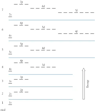
This order is shown as an energy-level diagram in Figure 1.14 (page 13). The orbitals fi ll in this order because the energy differences between the s,p,d, andf orbitals of the same principal quantum number become so great beyond
n52 that they overlap with the orbitals of the following principal quantum numbers. It is important to note that Figure 1.14 shows the fi lling order, not the order for any particular element. For example, for elements beyond zinc, electrons in the 3d orbitals are far lower in energy than those in the 4s orbitals. Thus, at this point, the 3d orbitals have become “inner” orbitals and have no role in chemical bonding. Hence, their precise ordering is unimportant.
Although these are the generalized rules, to illustrate how this delicate balance changes with increasing numbers of protons and electrons, the outer electrons in each of the Group 3 to Group 12 elements are listed here. These confi gurations are not important in themselves, but they do show how close the
ns and (n – 1)d electrons are in energy.
1.3 The Polyelectronic Atom
Atom Confi guration Atom Confi guration Atom Confi guration
Sc 4s23d1 Y 5s24d1 Lu 6s25d1
Ti 4s23d2 Zr 5s24d2 Hf 6s25d2
V 4s23d3 Nb 5s14d4 Ta 6s25d3
Cr 4s13d5 Mo 5s14d5 W 6s25d4
Mn 4s23d5 Tc 5s24d5 Re 6s25d5
Fe 4s23d6 Ru 5s14d7 Os 6s25d6
Co 4s23d7 Rh 5s14d8 Ir 6s25d7
Ni 4s23d8 Pd 5s04d10 Pt 6s15d9
Cu 4s13d10 Ag 5s14d10 Au 6s15d10
d-Block
La
Ac Th Pa U Np Pu Am Cm Bk Cf Es Fm Md No Ce Pr Nd Pm Sm Eu Gd Tb Dy Ho Er Tm Yb
f-Block
Sc Ti V Cr Mn Fe Co Ni Zn
Lr Rf Db Sg Bh Hs Mt Ds Rg Uub
Lu Hf Ta W Re Os Pt Au Hg Y Zr Nb Mo Tc Ru Pd Ag Cd
Cu
Ir Rh
p-Block
s-Block
Li
Na
Ca K
Rb
Cs
Fr Ra Ba Sr Mg
Be H He
Kr Br Se As Ge Ga Al
Ne F O N C B
Ar Cl S P Si
Uuo Uuh
Uup Uuq Uut
Tl Pb Bi Rn
Xe
At Po In Sn Sb Te I
13
Period
Energy
1 1s
2s
2p
3p
4p
5p
6p
7p
6d
5d
4d
4f
5f
3d
3s
4s
5s
6s
7s
7
6
5
4
3
2
1
FIGURE 1.14 Representation of the comparative energies of the atomic orbitals for fi lling order purposes.
For certain elements, the lowest energy is obtained by shifting one or both of the s electrons to d orbitals. Looking at the fi rst series in isolation would lead to the conclusion that there is some preference for a half-full or full set of
d orbitals by chromium and copper. However, it is more accurate to say that the inter-electron repulsion between the two s electrons is suffi cient in several cases to result in an s1 confi guration.
For the elements from lanthanum (La) to ytterbium (Yb), the situation is even more fl uid because the 6s, 5d, and 4f orbitals all have similar energies. For example, lanthanum has a confi guration of [Xe]6s25d1, whereas the next ele-ment, cerium, has a confi guration of [Xe]6s24f2. The most interesting electron confi guration in this row is that of gadolinium, [Xe]6s25d14f7, rather than the predicted [Xe]6s24f8. This confi guration provides more evidence of the impor-tance of inter-electron repulsion in the determination of electron confi guration
when adjacent orbitals have similar energies. Similar complexities occur among the elements from actinium (Ac) to nobelium (No), in which the 7s, 6d, and 5f
orbitals have similar energies.
1.4
Ion Electron Confi gurations
For the early main group elements, the common ion electron confi gurations can be predicted quite readily. Thus, metals tend to lose all the electrons in the outer orbital set. This situation is illustrated for the isoelectronic series (same electron confi guration) of sodium, magnesium, and aluminum cations:
Atom Electron confi guration Ion Electron confi guration
Na [Ne]3s1 Na1 [Ne]
Mg [Ne]3s2 Mg21 [Ne]
Al [Ne]3s23p1 Al31 [Ne]
Nonmetals gain electrons to complete the outer orbital set. This situation is shown for nitrogen, oxygen, and fl uorine anions:
Atom Electron confi guration Ion Electron confi guration
N [He]2s22p3 N32 [Ne]
O [He]2s22p4 O22 [Ne]
F [He]2s22p5 F2 [Ne]
Some of the later main group metals form two ions with different charges. For example, lead forms Pb21 and (rarely) Pb41. The 21 charge can be explained by the loss of the 6p electrons only (the “inert pair” effect, which we discuss in Chapter 9, Section 9.8), whereas the 41 charge results from loss of both 6s
and 6p electrons:
Atom Electron confi guration Ion Electron confi guration
Pb [Xe]6s24f145d106p2 Pb21 [Xe]6s24f145d10
Pb41 [Xe]4f145d10
Notice that the electrons of the higher principal quantum number are lost fi rst. This rule is found to be true for all the elements. For the transition metals, the s
electrons are always lost fi rst when a metal cation is formed. In other words, for the transition metal cations, the 3d orbitals are always lower in energy than the 4s orbitals, and a charge of 21, representing the loss of the two s electrons, is common for the transition metals and the Group 12 metals. For example, zinc always forms an ion of 21 charge:
Atom Electron confi guration Ion Electron confi guration