Fundamentals of Digital Image Processing

Fundamentals

of Digital

Image Processing

ANIL K. JAIN University of California, Davis

9

Image Analysis

and Computer Vision

9.1 INTRODUCTION

The ultimate aim in a large number of image processing applications (Table 9 . 1) is to extract important features from image data, from which a description, interpreta­ tion, or understanding of the scene can be provided by the machine (Fig. 9.1). For example, a vision system may distinguish parts on an assembly line and list theu features, such as size and number of holes. More sophisticated vision systems are

TABLE 9.1 Computer Vision Applications

1

Mail sorting, label reading, supermarket-product billing, bank-check processing, text reading

Tumor detection, measurement of size and shape of internal organs, chromosome analysis, blood cell count

Parts identification on assembly lines, defect and fault inspection

Recognition and interpretation of objects in a scene, motion control and execution through visual feedback

Map making from photographs, synthesis of weather maps Finger-print matching and analysis of automated security

systems

Target detection and identification, guidance of helicopters and aircraft in landing, guidance of remotely piloted vehicles (RPV), missiles and satellites from visual cues

Multispectral image analysis, weather prediction, classification and mon\totini of utban, aiticultutal, and matine

Preprocessing _extraction Feature Segmentation

Data analysis

---+---

Conclusion . , from analysis

I

I

Feature I Classification extraction and description

i

Image analysis system

Image understanding system

Symbolic representation

Figure 9.1 A computer vision system

Interpretation and description

able to interpret the results of analyses and describe the various objects and their relationships in the scene. In this sense image analysis is quite different from other image processing operations, such as restoration, enhancement, and coding, where the output is another image. Image analysis basically involves the study of feature

extraction, segmentation, and classification techniques (Fig. 9.2).

In computer vision systems such as the one shown in Fig. 9 . 1 , the input image is first preprocessed, which may involve restoration, enhancement, or just proper representation of the data. Then certain features are extracted for segmentation of the image into its components-for example, separation of different objects by extracting their boundaries. The segmented image is fed into a classifier or an image understanding system. Image classification maps different regions or segments into one of several objects, each identified by a label. For example, in sorting nuts and bolts, all objects identified as square shapes with a hole may be classified as nuts and those with elongated shapes, as bolts. Image understanding systems determine the relationships between different objects in a scene in order to provide its description. For example, an image understanding system should be able to send the report:

The field of view contains a dirt road surrounded by grass.

Such a system should be able to classify different textures such as sand, grass, or corn using prior knowledge and then be able to use predefined rules to generate a description.

I mage analysis techniques

Feature extraction Segmentation Classification

• Spatial features • Template matching • Clustering • Transform features • Thresholding • Statistical

• Edges and boundaries • Boundary detection • Decision trees • Shape features • Clustering • Similarity measures

• Moments • Ouad·trees • Min. spanning trees

• Texture • Texture matching

9.2 SPATIAL FEATURE EXTRACTION

Spatial features of an object may be characterized by its gray levels, their joint probability distributions, spatial distribution, and the like.

Amplitude Features

The simplest and perhaps the most useful features of an object are the amplitudes of its physical properties, such as reflectivity, transmissivity, tristimulus values (color), or multispectral response. For example, in medical X-ray images, the gray-level amplitude represents the absorption characteristics of the body masses and enables discrimination of bones from tissue or healthy tissue from diseased tissue. In infra­ red (IR) images amplitude represents temperature, which facilitates the segmenta­ tion of clouds from terrain (see Fig 7 . 10). In radar images, amplitude represents the

radar cross section, which determines the size of the object being imaged. Ampli­ tude features can be extracted easily by intensity window slicing or by the more general point transformations discussed in Chapter 7.

Histogram Features

Histogram features are based on the histogram of a region of the image. Let u be a random variable representing a gray level in a given region of the image. Define

( ) tJ,. p b[ _

] _ number of pixels with gray level x

Pu x = ro u -x _{- total number of pixels in the region' (9.1)}

x = O, . . . , L - l

Common features of Pu (x) are its moments, entropy, and so on, which are defined next.

L - l

Moments: m; = E

[

u;] =

x=O

L Xi Pu (x),

L-l

Absolute moments: m; = E[luli] = L lxliPu (x)

x=O

L-l

i = 1 , 2, . . . (9.2)

(9.3)

Central moments: µ; = E{[u - E(u)]'} = L (x

x =0

-m1Y Pu (x) (9.4)

L-1

Absolute central moments: µ; = E[lu - E(uW] = L Ix - m1l;Pu (x)

x=O

(9.5)

Entropy: H = E[-log2Pu]

L-l

(9.6) = - L Pu (x)

x=O

log2Pu (x) bits

Some of the eommon histogram features are dispersion = ili. mean = mi.

variance = µ2, mean square value or average energy = m2, skewness = µ3, kurtosis =

Often these features are measured over a small moving window W. Some of the histogram features can be measured without e�plicitly determining the histogram; for example,

m; (k, l) = N1 LL [u(m - k, n - l)Y (9.7)

w (m, n) E W

µ; (k, /) = Nl

LL

[u(m - k, n - I) - m1 (k, l)]i

w (m, n) E W (9.8)

where i = 1, 2, . . . and N,., is the number pixels in the window W. Figure 9.3 shows the spatial distribution of different histogram features measured over a 3 x 3 moving window. The standarq deviation emphasizes the strong edges in the image and dispersion feature extracts the fine edge structure. The mean, median, and mode extract low spatial-frequency features.

Second-order joint probabilities have also been found useful in applications such as feature extraction of textures (see Section 9.11). A second-order joint probability is defined as

Pu (xi. X2) �_{Pu 1,u2 (xi, X2)} �Prob[ U1 = Xi, U2 = X2], Xi, X2 = 0, ... , L - 1

number of pairs of pixels u1 = xi, u2 = X2 total number of such pairs of pixels in the region

Figure 9.3 Spatial distribution of histogram features measured over a 3 x 3 mov­ ing window. In each case, top to bottom and left to right, original image, mean, median, mode, standard deviation, and dispersion.

where u1 and u2 are the two pixels in the image region specified by some relation.

Image transforms provide the frequency domain information in the data. Transform features are extracted by zonal-filtering the image in the selected transform space (Fig. 9.4). The zonal filter, also called the feature mask, is simply a slit or an aper­ ture. Figure 9.5 shows different masks and Fourier transform features of different shapes. Generally, the high-frequency features can be used for edge and boundary detection, and angular slits can be used for detection of orientation. For example, an image containing several parallel lines with orientation 0 will exhibit strong energy along a line at angle -rr/2 + 0 passing through the origin of its two­ dimensional Fourier transform. This follows from the properties of the Fourier transform (also see the projection theorem, Section 10.4). A combination of an angular slit with a bandlimited low-pass, band-pass or high-pass filter can be used for discriminating periodic or quasiperiodic textures. Other transforms, such as Haar and Hadamard, are also potentially useful for feature extraction. However, systematic studies remain to be done to determine their applications. Chapters 5 and 7 contain examples of image transforms and their processed outputs.

Transform-feature extraction techniques are also important when the source data originates in the transform coordinates. For example, in optical and optical­ digital (hybrid) image analysis applications, the data can be acquired directly in the Fourier domain for real-time feature extraction in the focal plane.

I nput u(m, n) Forward

2�" B

�2 �2 �2

+

(a) Slits and apertures (b) Rectangular 'and circular shapes

(c) Triangular and vertical shapes (d) 45° orientation and the letter J

Figure 9.5 Fourier domain features.

9.4 EDGE DETECTION

A problem of fundamental importance in image analysis is edge detection. Edges characterize object boundaries and are therefore useful for segmentation, registra­ tion, and identification of objects in scenes. Edge points can be thought of as pixel locations of abrupt gray-level change. For example, it is reasonable to define edge points in binary images as black pixels with at least one white nearest neighbor, that is, pixel locations (m, n) such that u(m, n) = 0 and g(m, n) = 1, where

y

Figure 9.6 Gradient of f(x, y) along r direction.

where E9 denotes the logical exclusive-OR operation. For a continuous image

f(x, y) its derivative assumes a local maximum in the direction of the edge. There­ fore, one edge detection technique is to measure the gradient of f along r in a direction 8 (Fig. 9.6), that is,

af af ax af ay .

- = -_{ar ax ar ay a}- + - - = f, _r .t cos 8 + J; sm 0 y (9.11)

The maximum value of af/ar is obtained when (a/a0)(a//ar) = 0. This gives

-f .. sin 08 +fr cos 08 = 0 => 08 = tan-1

(

I

)

(

af

)

_n

ar max

(9.12a)

(9.12b)

where 88 is the direction of the edge. Based on these concepts, two types of edge detection operators have been introduced [6-11], gradient operators and compass operators. For digital images these operators, also called masks, represent finite­ difference approximations of either the orthogonal gradients fx,/y or the directional gradient aflar. Let H denote a p x p mask and define, for an arbitrary image U, their inner product at location (m, n) as the correlation

(U, H)m, n

� LL

h (i, j)u(i + m, j + n) = u(m, n) ® h(-m, -n) (9. 13)

i j

Gradient Operators

These are represented by a pair of masks Hi . H2, which measure the gradient of the image u (m, n) in two orthogonal directions (Fig. 9. 7). Defining the bidirectional gradients g1 (m, n)

�

(U, H1 )m, n, g2 (m, n)

�

(U, H2 )m, n the gradient vector magnitude and direction are given by

g(m, n) = n) + gHm, n) (9. 14)

( ) - _1g2 (m, n)

08 m, n -tan

( )

u(m, n)

Figure 9.7 Edge detection via gradient operators.

Often the magnitude gradient is calculated as

g(m, n) � _{lg1 (m, n)I + lg2 (m, n)I} especially when implemented in digital hardware.

Table 9.2 lists some of the common gradient operators. The Prewitt, Sobel, and isotropic operators compute horizontal and vertical differences of local sums. This reduces the effect of noise in the data. Note these operators have the desirable property of yielding zeros for uniform regions.

The pixel location (m, n) is declared an edge location if g(m, n) exceeds some threshold t. The locations of edge points constitute an edge map e(m, n), which is defined as

The edge map gives the necessary data for tracing the object boundaries in an image. Typically, t may be selected using the cumulative histogram of g(m, n) so

TABLE 9.2 Some Common Gradient Operators.

Boxed element indicates the location of the origin

(a) Sobel (b) Kirsch

(c) Stochastic 5 x 5 (d) Laplacian

Figure 9.8 Edge detection examples. In each case, gradient images (left), edge maps (right).

that 5 to 10% of pixels with largest gradients are declared as edges. Figure 9.8a shows the gradients and edge maps using the Sobel operator on two different images.

Compass Operators

u(m, n) _{gK (m, n)}

hk (-m, -n) Max {I · I}

k

Gradient g(m, n) 1 Edge map

1 1 1 i

0 0 0 (N)

IJ k Threshold

Figure 9.9 Edge detection via compass operators.

1 1 0 "\ 1 0 -1 � 0 - 1 -1 ,/

1 0 - 1 (NW) 1 0 -1 (W) 1 0 - 1 (SW)

-1 - 1 -1 0 -1 -1 1 0 -1 1 1 0

-1 - 1 - 1 t - 1 - 1 0 \.i -1 0 1 � 0 1 1 /'

0 0 0 (S) -1 0 1 (SE) -1 0 1 (E) -1 0 1 (NE)

1 1 1 0 1 1 -1 0 1 -1 -1 0

Let gk (m, n) denote the compass gradient in the direction 0k = -rr/2 + k-rr/4, k = 0, . . . , 7. The gradient at location (m, n) is defined as

g(m, n)

�

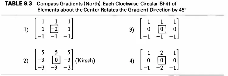
max_k {lgk (m, n)I} (9.19) which can be thresholded to obtain the edge map as before. Figure 9.8b shows the results for the Kirsch operator. Note that only four of the preceding eight compass gradients are linearly independent. Therefore, it is possible to define four 3 x 3 arrays that are mutually orthogonal and span the space of these compass gradients. These arrays are called orthogonal gradients and can be used in place of the compass gradients [12]. Compass gradients with higher angular resolution can be designed by increasing the size of the mask.

TABLE 9.3 Compass Gradients (North). Each Clockwise Circular Shift of Elements about the Center Rotates the Gradient Direction by 45°

1) [ �

-1 -1 -1

81

�i

_'l

u � -�l

2)

[-;

@J

_;](Kirsch)

-3 -3 -3

[ 1

2

1]

4)

-� � -�

Laplace Operators and Zero Crossings

The foregoing methods of estimating the gradients work best when the gray-level transition is quite abrupt, like a step function. As the transition region gets wider (Fig. 9.10), it is more advantageous to apply the second-order derivatives. One frequently encountered operator is the Laplacian operator, defined as

f(x)

df dx

Double edge

crossing

(a) First and second derivatives for edge detection

(b) An image and its zero-crossings.

Figure 9.10 Edge detection via zero­ crossings.

Table 9.4 gives three different discrete approximations of this operator. Figure 9.8d shows the edge extraction ability of the Laplace mask (2). Because of the second­ order derivatives, this gradient operator is more sensitive to noise than those pre­ viously defined. Also, the thresholded magnitude of V'2 f produces double edges. For these reasons, together with its inability to detect the edge direction, the Laplacian as such is not a good edge detection operator. A better utilization of the Laplacian is to use its zero-crossings to detect the edge locations (Fig. 9. 10). A generalized Laplacian operator, which approximates the Laplacian of Gaussian functions, is a powerful zero-crossing detector [13]. It is defined as

li

[

( m 2 + n

(

m 2 + n 2

)

h(m, n)

=

c 1

-a2 exp - 2a2 (9.21)

TABLE 9.4 Discrete Laplace Operators fore, the zero-crossings detector is equivalent to a low-pass filter having a Gaussian impulse response followed by a Laplace operator. The low-pass filter serves to attenuate the noise sensitivity of the Laplacian. The parameter CT controls the amplitude response of the filter output but does not affect the location of the zero-crossings.

Directional information of the edges can be obtained by searching the zero­ crossings of the second-order derivative along r for each direction 0. From (9.11), we obtain

Zero-crossings are searched as 0 is varied [14]. Stochastic Gradients [16]

The foregoing gradient masks perform poorly in the presence of noise. Averaging, low-pass filtering, or least squares edge fitting [15] techniques can yield some reduction of the detrimental effects of noise. A better alternative is to design edge extraction masks, which take into account the presence of noise in a controlled manner. Consider an edge model whose transition region is 1 pixel wide (Fig. 9.11).

u( m, n)

To detect the presence of an edge at location P, calculate the horizontal gradient, for instance, as

g1(m,n)�u1(m, n - l)-ub(m,n

+ 1) (9.23)

Here

u1(m, n)

and

ub(m, n)

are the optimum forward and backward estimates of

u(m,

n) based on the noisy observations given over some finite regions W of the left­

and right half-planes, respectively. Thus

u1(m, n)

and

uh (m,

n) _{are semicausal esti­}

mates (see Chapter 6). For observations

v (m, n)

containing additive white noise, we can find the best linear mean square semicausal FIR estimate of the form

u,(m, n) �

2:2:

a(k, l)v(m

- k,

n -l),

w = [(k, /): lk l :=;p, 0 :=; [ $ q] (9.24)

(k, l) E W

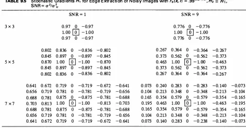
The filter weights a (k, /) can be determined following Section 8.4 with the modification that W is a semicausal window. [See (8.65) and (8.69)]. The backward semicausal estimate employs the same filter weights, but backward. Using the definitions in (9.23), the stochastic gradient operator H1 is obtained as shown in Table 9.5. The operator H2 would be the 90° counterclockwise rotation of Hi. which, due to its symmetry properties, would simply be H{. These masks have been normalized so that the coefficient a (0, 0) in (9.24) is unity. Note that for high SNR the filter weights decay rapidly. Figure 9.8c shows the gradients and edge maps obtained by applying the 5 x 5 stochastic masks designed for SNR = 9 but applied to noiseless images. Figure 9.12 compares the edges detected from noisy images by the Sobel and the stochastic gradient masks.

Performance of Edge Detection Operators

Edge detection operators can be compared in a number of different ways. First, the image gradients may be compared visually, since the eye itself performs some sort of edge detection. Figure 9.13 displays different gradients for noiseless as well as noisy images. In the noiseless case all the operators are roughly equivalent. The stochastic gradient is found to be quite effective when noise is present. Quantitatively, the performance in noise of an edge detection operator may be measured as follows. Let

n0

be the number of edge pixels declared and

n1

be number of missed or new edge pixels after adding noise. If n0 is held fixed for the noiseless as well as noisy images, then the edge detection error rate is

P. ₌

n1

e

no

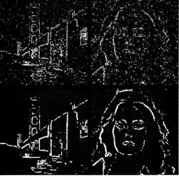
(9.25)

In Figure 9.12 the error rate for the Sobel operator used on noisy images with SNR = 10 dB is 24%, whereas it is only 2% for the stochastic operator.

Another figure of merit for the noise performance of edge is the quantity

Figure 9.12 Edge detection from noisy images. Upper two, Sobel. Lower two, stochastic.

where d; is the distance between a pixel declared as edge and the nearest ideal edge pixel, a is a calibration constant, and N1 and Nn are the number of ideal and detected edge pixels respectively. Among the gradient and compass operators of Tables 9.2 and 9.3 (not including the stochastic masks), the Sobel and Prewitt operators have been found to yield the highest performance (where performance is proportional to the value of P) [17] .

Line and Spot Detection

(a) Gradients for noiseless image (b) Gradients for noisy i mage

Figure 9.13 Comparison of edge extraction operators. In each case

Hffi

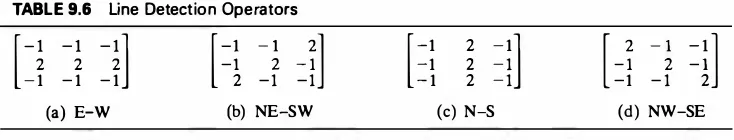
the operators are (1) smoothed gradient, (2) sobel, (3) isotropic, (4) semicausal model based 5 x 5 stochastic. Largest 5% of the gradient magnitudes were declared edges.

TABLE 9.6 Line Detection Operators

[-i

-1 -1 -1 [=�

-

i

-

i]

-l

-i]

2 - 1 - 1

[-1

-1 -1

2

-1]

2 - 1

2 - 1

[-i

-1

-l

- 1

=�]

2

(a) E-W (b) NE-SW (c) N-S (d) NW-SE

Spots are isolated edges. These are most easily detected by comparing the value of a pixel with an average or median of the neighborhood pixels.

9.5 _{BOUNDARY EXTRACTION}

Boundaries are linked edges that characterize the shape of an object. They are useful in computation of geometry features such as size or orientation.

Connectivity

Conceptually, boundaries can be found by tracing the connected edges. On a rec­ tangular grid a pixel is said to be four- or eight-connected when it has the same properties as one of its nearest four or eight neighbors, respectively (Fig. 9.14). There are difficulties associated with these definitions of connectivity, as shown in Fig. 9. 14c. Under four-connectivity, segments 1, 2, 3, and 4 would be classified as disjoint, although they are perceived to form a connected ring. Under eight­ connectivity these segments are connected, but the inside hole (for example, pixel

(a) (b)

2

3

(c)

Figure 9.14 Connectivity on a rectangular grid. Pixel A and its (a) 4-connected and (b) 8-connected neighbors; (c) connectivity paradox: "Are B and C con­ nected?"

be avoided by considering eight-connectivity for object and four-connectivity for background. An alternative is to use triangular or hexagonal grids, where three- or six-connectedness can be defined. However, there are other practical difficulties that arise in working with nonrectangular grids.

Contour Following

As the name suggests, contour-following algorithms trace boundaries by ordering successive edge points. A simple algorithm for tracing closed boundaries in binary

images is shown in Fig. 9.15. This algorithm can yield a coarse contour, with some of

the boundary pixels appearing twice. Refinements based on eight-connectivity tests

for edge pixels can improve the contour trace [2]. Given this trace a smooth curve,

such as a spline, through the nodes can be used to represent the contour. Note that

this algorithm will always trace a boundary, open or closed, as a closed contour. This

method can be extended to gray-level images by searching for edges in the 45° to

135° direction from the direction of the gradient to move from the inside to the

outside of the boundary, and vice-versa (19). A modified version of this contour­

following method is called the crack-following algorithm [25]. In that algorithm each

pixel is viewed as having a square-shaped boundary, and the object boundary is traced by following the edge-pixel boundaries.

Edge Linking and Heuristic Graph Searching [18-21]

A boundary can also be viewed as a path through a grapl) formed by linking the edge elements together. Linkage rules give the procedure for connecting the edge

elements. Suppose a graph with node locations xk. k = 1, 2, . .. is formed from node

A to node B. Also, suppose we are given an evaluation function <l>(xk), which gives the value of the path from A to B constrained to go through the node xk. In heuristic search algorithms, we examine the successors of the start node and select the node that maximizes <!>( · ). The selected node now becomes the new start node and the

consti-29 28

Algorithm

1 . Start i nside A (e.g., 1 )

2. Turn left and step to next pixel if in region A, (e.g., 1 to 2), otherwise turn right and step (e.g., 2 to 3) 3. Continue until arrive at starting

point 1

Figure 9.15 Contour following in a binary image.

tutes the boundary path. The speed of the algorithm depends on the chosen <l>( ·) [20, 21]. Note that such an algorithm need not give the globally optimum path.

Example 9.2 Heuristic search algorithms [19]

Consider a 3 x 5 array of edges whose gradient magnitudes lg I and tangential contour

directions 0 _{are shown in Fig. 9.16a. The contour directions are at 90° to the gradient} directions. A pixel X is considered to be linked to Y if the latter is one of the three eight-connected neighbors (Yi, Yi, or YJ in Fig. 9.16b) in front of the contour direction and if l0(x) -0(y)I < 90°. This yields the graph of Fig. 9.16c.

As an example, suppose cj>(xk) is the sum of edge gradient magnitudes along the path from A to xk. _{At A, the successor nodes are D, C, and G, with cj>(D)} = _12,

cj>(C) = 6, and cj>(G) = 8. Therefore, node D is selected, and C and G are discarded. From here on nodes E, F, and B provide the remaining path. Therefore, the boundary path is ADEFB. On the other hand, note that path ACDEFB is the path of maximum cumulative gradient.

Dynamic Programming

Dynamic programming is a method of finding the global optimum of multistage pro­ cesses. It is based on Bellman's principal of optimality [22], which states that the

5

-�

y

5

�

-y �

3 2 3

- -

-(a) Gradient magnitudes contour directions

6

-(b) Linkage rules (c) Graph interpretation

Figure 9.16 Heuristic graph search method for boundary extraction.

on the path. Thus if C is a point on the optimum path between A and B (Fig. 9.17), then the segment CB is the optimum path from C to B, no matter how one arrives

at C.

To apply this idea to boundary extraction [23], suppose the edge map has been converted into a forward-connected graph of N stages and we have an evaluation function

N N N

S (xi, Xz, . . . , xN, N)

� L

lg(xk)I - a L l0(xk) - 0(xk - 1)l -l3 L d(xb Xk - 1) (9.27)

k = I k = 2 k = 2

Here xh k = 1, . . . , N represents the nodes (that is, the vector of edge pixel loca­ tions) in the kth stage of the graph, d ( x, y) is the distance between two nodes x and

y; lg (xk)I , 0(xk) are the gradient magnitude and angles, respectively, at the node xb

and a and 13 are nonnegative parameters. The optimum boundary is given by connecting the nodes xk, k = 1, . . . , N, so that S (:Xi. x2, • • • , iN, N) is maximum. Define

cf>(xN, N)

�

max {S (xi. . . . , XN, N)}

•1 · · · •N - 1

(9.28) Using the definition of (9.27), we can write the recursion

S(xi. . . . , xN, N) = S (xi. . . . , XN-i . N -1)

+ {lg (xN)I - al0(xN) - 0(xN - 1)I - j3d (xN, XN- 1)}

�

S (xi. . . . , XN- i. N - 1) + f(XN- i . xN)

(9.29)

where f(xN-i. xN) represents the terms in the brackets. Letting N = k in (9.28) and (9.29), it follows by induction that

XI • . • Xk - 1

k = 2, . . . ,N

(9.30)

'k -I

S (:ii . . . . , :iN, N) = max {<I>(xN, N)}

'N <I>(xi . 1)

�

lg (x1)I

This procedure is remarkable in that the global optimization of S (x1 , • • • , XN, N) has been reduced to N stages of two variable optimizations. In each stage, for each value of xk one has to search the optimum <l>(xt. k). Therefore, if each xk takes L different values, the total number of search operations is (N - l)(L 2 -1) + (L -1). This would be significantly smaller than the L N -1 exhaustive searches required for direct maximization of S (x2, x2, • • • , xN, N) when L and N are large.

Example 9.3

Consider the gradient image of Fig. 9.16. Applying the linkage rule of Example 9.2 and letting o: = 4hr, 13 = 0, we obtain the graph of Fig. 9.18a which shows the values

of various segments connecting different nodes. Specifically, we have N = 5 and

<l>(A, 1) = 5. For k = 2, we get

<l>(D, 2) = max(ll, 12) = 12

which means in arriving at D, the path ACD is chosen. Proceeding in this manner some of the candidate paths (shown by dotted lines) are eliminated. At k = 4, only two paths are acceptable, namely, ACDEF and AGHJ. At k = 5, the path JB is eliminated,

giving the optimal boundary as ACDEFB.

cf>(x •• kl

D E F

max ( 1 1 , 12) (161 (23)

B

Q

(51 (8) _{max ( 1 9, 28)}

A

(al Paths with values

,, ,,"' ,,,,

(8) max (8, 10) max ( 1 3, 101

G H J

2 3 4

(bl cf>(x •• kl at various stages. Solid line gives the optimal path.

Figure 9.18 Dynamic programming for optimal boundary extraction.

B

y 8

• (s, 8 )

(a) Straight line (b) Hough transform

Figure 9.19 The Hough transform.

Hough Transform [1 , 24]

A straight line at a distance s and orientation 8 (Fig. 9 .19a) can be represented as

s = x cos 8 + y sin 8 (9.31)

The Hough transform of this line is just a point in the (s, 8) plane; that is, all the points on this line map into a single point (Fig. 9. 19b ). This fact can be used to detect straight lines in a given set of boundary points. Suppose we are given bound­ ary points (x;, y;), i = 1 , . . . , N. For some chosen quantized values of parameters s and 8, map each (x;, y;) into the (s, 8) space and count C(s, 8), the number of edge points that map into the location (s, 8), that is, set

(9.32)

Then the local maxima of C(s, 8) give the different straight line segments through the edge points. This two-dimensional search can be reduced to a one-dimensional search if the gradients 8; at each edge location are also known. Differentiating both sides of (9.31) with respect to x, we obtain

��

= -cot 8 = tan

(�

+ 8

)

(9.33) Hence C(s, 8) need be evaluated only for 8 = -rr/2 -8;. The Hough transform can also be generalized to detect curves other than straight lines. This, however, increases the dimension of the space of parameters that must be searched [3] . From Chapter 10, it can be concluded that the Hough transform can also be expressed as the Radon transform of a line delta function.

9.6 _{BOUNDARY REPRESENTATION}

environmental modeling of aircraft-landing testing and training, and other com­ puter graphics problems.

Chain Codes [26]

In chain coding the direction vectors between successive boundary pixels are en­ coded. For example, a commonly used chain code (Fig. 9.20) employs eight direc­ tions, which can be coded by 3-bit code words. Typically, the chain code contains the start pixel address followed by a string of code words. Such codes can be generalized by increasing the number of allowed direction vectors between successive boundary pixels. A limiting case is to encode the curvature of the contour as a function of contour length t (Fig. 9.21).

3

A

2

2

6 7

4

(b) Contour

Boundary pixel orientations: (A). 7601 065543242 1

Chain code: A 1 1 1 1 1 0 000 001 000 1 1 0 101 101 1 1 0 01 1 010 1 00 010 001

Figure 9.20 Chain code for boundary representation.

y _II

Algorithm:

1 . Start at any boundary pixel, A.

2. Find the nearest edge pixel and code its orientation. In case of a tie, choose the one with largest

(or smallest) code value.

3. Continue until there are no more boundary pixels.

(a) Contour (b) () vs. t curve. Encode 8(t).

Fitting Line Segments [1]

Straight-line segments give simple approximation of curve boundaries. An interest­ ing sequential algorithm for fitting a curve by line segments is as follows (Fig. 9.22).

Algorithm. Approximate the curve by the line segment joining its end points

(A, B ). If the distance from the farthest curve point (C) to the segment is greater than a predetermined quantity, join AC and BC. Repeat the procedure for new segments AC and BC, and continue until the desired accuracy is reached.

8-Spline Representation [27-29]

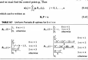
B -splines are piecewise polynomial functions that can provide local approximations of contours of shapes using a small number of parameters. This is useful because human perception of shapes is deemed to be based on curvatures of parts of contours (or object surfaces) [30]. This results in compression of boundary data as well as smoothing of coarsely digitized contours. B -splines have been used in shape synthesis and analysis, computer graphics, and recognition of parts from bound­ aries.

Let t be a boundary curve parameter and let x (t) and y (t) denote the given boundary addresses. The B -spline representation is written as

n

x(t) = L p; B;, k (t) i = 0

x(t)

�

[x (t), y (t) y,

(9.34)

where p; are called the control points and the B;, k (t), i = 0, 1 , ... , n, k = 1 , 2 . . . are called the normalized B-splines of order k. In computer graphics these functions are also called basis splines or blending functions and can be generated via the recursion

( ) Li (t - t;)B;,k- 1 (t) (t;+k - t)B;+ 1.k- 1 (t) ( )

B; ' k t = _{t; + k} + _{) ,} k = 2, 3, . . . 9.35a

-I -f; (t; + k - t; + I

B· '· 1 _{(t) �}

{

l, t; =5 t < .t;+1 0, otherwise _(9.35b)

where we adopt the convention 0/0

�

0. The parameters t;, i = 0, 1 , . . . are called the

knots. These are locations where the spline functions are tied together. Associated

E

( 1 ) (2) (3)

B;, 2 (t)

with the knots are nodes S;, _{which are defined as the mean locations of successive}

k -1 knots, that is, a 1

S; ₌

k -l (t;+ J + l;+ 2 + · · · + t;+ k-J), 0 ::5 i ::5 n, k ?:. 2 (9.36)

The variable t is also called the node parameter, of which t; and S; are special values. Figure 9.23 shows some of the B -spline functions. These functions are nonnegative and have finite support. In fact, for the normalized B -splines, 0 ::5 B;, k (t) ::5 1 and the region of support of B;, k (t) is [t;, t; + k). The functions B;, k (t) form a basis in the space of piecewise-polynomial functions. These functions are called open B-splines or

closed (or periodic) B-splines, depending on whether the boundary being repre­ sented is open or closed. The parameter k controls the order of continuity of the curve. For example, for k = 3 the splines are piecewise quadratic polynomials. For k = 4, these are cubic polynomials. In computer graphics k = 3 or 4 is generally found to be sufficient.

When the knots are uniformly spaced, that is,

f; + 1 -f; = Llt, Vi (9.37a) the B;,k (t) are called uniform splines and they become translates of Bo,k (t), that is,

B;,k (t) = Bo,k (t - i), i = k - 1, k, _.._. , n -k + _{1 (9.37b)} Near the boundaries B;,k (t) is obtained from (9.35). For uniform open B -splines with Llt = 1 , the knot values can be chosen as

t; =

(�

-k + 1 n -k+2

i < k k ::5 i ::5 n i > n

and for uniform periodic (or closed) B -splines, the knots can be chosen as

t; = imod(n + 1)

B;, k (t) = _{Bo,k[(t - i)}mod(n + 1)] B;, 1 (t)

(9.38)

(9.39)

(9.40)

1

Constant

- t

t,- + 1

For k = 1 , 2, 3, 4 and knots given by (9.39), the analytic forms of Bo.k(t) are pro­ vided in Table 9.7.

Control points. The control points p; are not only the series coefficients in (9.34), they physically define vertices of a polygon that guides the splines to trace a smooth curve (Fig. 9.24). Once the control points are given, it is straightforward to obtain the curve trace x(t) via (9.34). The number of control points necessary to reproduce a given boundary accurately is usually much less than the number of points needed to trace a smooth curve. Data compression by factors of 10 to 1000 can be achieved, depending on the resolution and complexity of the shape.

A B -spline-generated boundary can be translated, scaled (zooming or shrink­ ing), or rotated by performing corresponding control point transformations as follows:

Translation: _p; = _p; + _{Xo, Xo =} [xo,YoY (9.41)

(a) (b) original boundaries containing 1038 and 10536 points respectively to yield indistin­ guishable reproduction: (c), (d) corresponding 16 and 99 control points respec­ tively. Since (a), (b) can be reproduced from (c), (d), compression ratios of greater than 100 : 1 are achieved.

where Bk> P, and x are (n + 1) x (n + 1), (n + 1) x 2, and (n + 1) x 2 matrices of elements B;, k (si), p;, x(si) respectively. When si are the node locations the matrix Bk

is guaranteed to be nonsingular and the control-point array is obtained as

Example 9.4 Quadratic B-splines, k = 3

(a)

Periodic case:

From (9.36) and (9

.3

9) the nodes (sampling locations) are

[s s s s ]

_{0' J , 2'} =

[�

,

�

,

2

, . . . , 2n - 1

,

�

l]

• • .

,

" 2 2 2

2 2 2

Then from (9.47), the blending function

Bo.3

(t)

gives the circulant matrix

(b)

Nonperiodic case:

From (9.36) and (9

.3

8) the knots and nodes are obtained as

[t0,li, .. . ,ln+3]

=

[0,0,0, 1,2,3, . . . ,n -2,n - 1,n - 1,n - 1]

[

1 3

5

7

2n - 3

J

[s s s ] =

O , J , . • . , n o _ , _ , _ , _ , . . . , __

,n - 1

'2 2 2 2

2

The nonperiodic blending functions for

k = 3

are obtained as

(-�

(t -

�y

+

�'

B1,3(t) =

�

(

t - 2

)

2

,

0,

0 st <j - 2

�

(t

-j

+

2

)

2

,

j - 2 st < j -

1

(

1)2 3

j

- 1

-5,_

t <

j

Bi.3(t) =

_{- t -j +l +4,}

� (t -j - 1)2,

j -:5. t <j + l

0,

0,

j + 1 st s n - 1, j

=

_{2, 3, .. . , n -}

2

0,

-� (t - n +

3)2, -�

₂

(t - n

+ �

_{3 3}

)

2 +

�'

O s t <n - 3

n - 3 s t < n - 2

n - 2st sn - 1

B

n,3 ( ) -

1 _

{

O,

0 -:5. t < n - 2

(t - n + 2)2, n -2-:5.t-:5.n - 1

From these we obtain

n + 1

8

2 5 1 0

1 6 1

""""""""" n + 1 1 6 1

0 1 5 2

Figure 9.25 shows a set of uniformly sampled spline boundary points x (s1), j = 0, . .. , 13. Observe that the sh and not x (s;),y (s;), are required to be uniformly

spaced. Periodic and open quadratic B-spline interpolations are shown in Fig. 9.25b and c. Note that in the case of open B-splines, the endpoints of the curve are also control points.

The foregoing method of extracting control points from uniformly sampled boundaries has one remaining difficulty-it requires the number of control points be equal to the number of sampled points. In practice, we often have a large number of finely sampled points on the contour and, as is evident from Fig. 9.24, the number of control points necessary to represent the contour accurately may be much smaller. Therefore, we are given x(t) for t = � 0, � 1, • • • , � m, where m 'P n. Then we have an overdetermined (m + 1) x (n + 1) system of equations

n

x(�j) = L Bi, k (�j) Pi, j = 0, . . . , m (9.48)

i = O

Least squares techniques can now be applied to estimate the control points Pi·

With proper indexing of the sampling points �j and letting the ratio (m + 1)/(n + 1)

(a) (b)

Control points

.. / �.

•.

..

(c)

be an integer, the least squares solution can be shown to require inversion of a circulant matrix, for which fast algorithms are available [29].

Fourier Descriptors

Once the boundary trace is known, we can consider it as a pair of waveforms

x (t), y (t). Hence any of the traditional one-dimensional signal representation tech­ niques can be used. For any sampled boundary we can define

u (n) � x(n) + jy(n), n = O, l, . . . ,N - l (9.49)

which, for a closed boundary, would be periodic with period N. Its DFf repre­ sentation is

The complex coefficients a (k) are called the Fourier descriptors (FDs) of the bound­ ary. For a continuous boundary function, u(t), defined in a similar manner to (9.49), the FDs are its (infinite) Fourier series coefficients. Fourier descriptors have been found useful in character recognition problems [32].

Effect of geometric transformations. Several geometrical transforma­ tions of a boundary or shape can be related to simple operations on the FDs (Table

9.8). If the boundary is translated by

fl. .

Uo

=

Xo

+ JYo (9.51)

then the new FDs remain the same except at k = 0. The effect of scaling, that is, shrinking or expanding the boundary results in scaling of the a (k). Changing the starting point in tracing the boundary results in a modulation of the a (k). Rotation of the boundary by an angle 00 causes a constant phase shift of 00 in the FDs. Reflection of the boundary (or shape) about a straight line inclined at an angle e (Fig. 9.26),

Ax + By + C = O

TABLE 9.8 Properties of Fou rier Descriptors

c A

y

Figure 9.26 Reflection about a straight

line.

gives the new boundary i (n),y (n) as (Problem 9.11) it (n) = u* (n)ei20 + 2'Y

where

a -(A + jB)C

'Y = _{A 2 + B2 '} exp(j26) = _{A 2 + B2}

(9.53)

For example, if the line (9.52) is the x -axis, that is, A = C = 0, then 6 = 0, 'Y = 0 and the new FDs are the complex conjugates of the old ones.

Fourier descriptors are also regenerative shape features. The number of de­ scriptors needed for reconstruction depends on the shape and the desired accuracy. Figure 9.27 shows the effect of truncation and quantization of the FDs. From Table 9.8 it can be observed that the FD magnitudes have some invariant properties. For example Ja (k)J, k = 1 , 2, . . . , N - 1 are invariant to starting point, rotation, and reflection. The features a (k)!Ja (k)J are invariant to scaling. These properties can be used in detecting shapes regardless of their size, orientation, and so on. However, the FD magnitude or phase alone are generally inadequate for reconstruction of the original shape (Fig. 9.27).

Boundary matching. The Fourier descriptors can be used to match similar shapes even if they have different size and orientation. If a (k) and b (k) are the FDs of two boundaries u ( n) and v ( n ), respectively, then their shapes are similar if the distance

{N-1

}

d(u

o

, a, 60, no) �

uo���,60

_n�o

Ju(n) - av(n + n0)ei0o - u0 J2 (9.54)

59. 1 3

F D real part

-59. 1 3 1

69.61

FD imaginary part

0

(a)

-69.61 1

(b)

(c) (d)

(e) (f)

Figure 9.27 Fourier descriptors. (a) Given shape; (b) FDs, real and imaginary components; (c) shape derived from largest five FDs; (d) derived from all FDs quantized to 17 levels each; (e) amplitude reconstruction; (f) phase reconstruction.

1 28

minimum when

ito = O

L

c(k) _{cos(i!Jk + k<I> + 80)}

k

L

_k lb(k)l2 _(9.55)

and

L

c (k) _{sin( i!Jk + k<I>)}

k

tan 90 = -

L

c (k) _{cos(i!Jk + k<!>)}

k

where a (k)b* (k) = c(k)ei"1k, <!>

� -2-rrn0/N,

and c (k) is a real quantity. These equa­ tions give a and 90, from which the minimum distance d is given by

d = min [d(<!>)] = min

{L

la(k) - ab(k) exp[j(k<!> + 90)]12

}

(9.56)

4> 4> k

The distance d ( <!>) can be evaluated for each <!> = <!>( n0), n0 = 0, 1, . . . , N - 1 and the minimum searched to obtain d. The quantity d is then a useful measure of difference between two shapes. The FDs can also be used for analysis of line patterns or open curves, skeletonization of patterns, computation of area of a surface, and so on (see Problem 9 .12).

Instead of using two functions x (t) and y (t), it is possible to use only one function when t represents the arc length along the boundary curve. Defining the arc tangent angle (see Fig. 9.21)

- -l

[

dy(t)!dt

]

9(t) -tan _dx(t)/dt (9.57)

the curve can be traced if x (0), y (0), and 9(t) are known. Since t is the distance along the curve, it is true that

dt2 = dx2 + dy2 =>

(��r

+

('ZY

= l

which gives dx/dt = cos9(t), dyldt = sin 9(t), or

x(t) = x(O) +

J:

[

�:

:g1]

dT

Sometimes, the FDs of the curvature of the boundary

or those of the detrended function

( ) A d9(t) K t = dt

A A

J'

2-rrt

9 (t) = O K(T)dT -T

(9.58)

(9.59)

(9.60)

are used [31]. The latter has the advantage that 0 (t) does not have the singularities at corner points that are encountered in polygon shapes. Although we have now only a real scalar set of FDs, their rate of decay is found to be much slower than those of u (t).

Autoregressive Models

If we are given a class of object boundaries-for instance, screwdrivers of different sizes with arbitrary orientations-then we have an ensemble of boundaries that could be represented by a stochastic model. For instance, the boundary coordinates

x (n),y(n) could be represented by AR processes (33]

p independent, so that the coordinates x1 (n) and x2 (n) can be processed indepen­ dently. For closed boundaries the covariances of the sequences {x; (n)}, i = 1 , 2 will be periodic. The AR model parameters a; (k), 137, and µ; can be considered as

features of the given ensemble of shapes. These features can be estimated from a given boundary data set by following the procedures of Chapter 6.

Properties of AR features. Table 9.9 lists the effect of different geometric transformations on the AR model parameters. The features a; (k) are invariant under translation, scaling, and starting point. This is because the underlying corre­ lations of the sequences x; (n), which determine the a;(k), are also invariant under these transformations. The feature 137 is sensitive to scaling and f.L; is sensitive to scaling as well as translation. In the case of rotation the sum la1 (k)l2 + la2 (k)l2 can be shown to remain invariant.

AR models are also regenerative. Given the features {a; (k), µ;, 137} and the

residuals e; (k), the boundary can be reconstructed. The AR model, once identified

for a class of objects, can also be used for compression of boundary data,

x1 (n),x1 (n) via the DPCM method (see Chapter 11).

9.7 REGION REPRESENTATION

The shape of an object may be directly represented by the region it occupies. For example, the binary array

u (m n) ='

{

l , _{0, otherwise} if (m , �) E � (9.63)

is a simple representation of the region Y£ . Boundaries give an efficient representa­ tion of regions because only a subset of u (m, n) is stored. Other forms of region representation are discussed next.

Run-length Codes

Any region or a binary image can be viewed as a sequence of alternating strings of Os and ls. Run-length codes represent these strings, or runs. For raster scanned regions, a simple run-length code consists of the start address of each string of ls (or Os), followed by the length of that string (Fig. 9.28). There are several forms of run-length codes that are aimed at minimizing the number of bits required to represent binary images. Details are discussed in Section 11.9. The run-length codes have the advantage that regardless of the complexity of the region, its representa­ tion is obtained in a single raster scan. The main disadvantage is that it does not give the region boundary points ordered along its contours, as in chain coding. This makes it difficult to segment different regions if several are present in an image.

Quad-trees [34]

In the quad-tree method, the given region is enclosed in a convenient rectangular area. This area is divided into four quadrants, each of which is examined if it is

0 2 3

0

2 3 4

(a) Binary image

4 Run-length code ( 1 , 1 ) 1 , ( 1 , 3)2 (2, 0)4

(3, 1 )2

Run # 1 , 2

3 4

totally black (ls) or totally _white (Os). The quadrant that has both black as well as white pixels is called gray and is further divided into four quadrants. A tree struc­ ture is generated until each subquadrant is either black only or white only. The tree can be encoded by a unique string of symbols b (black), w (white), and g (gray), where each g is necessarily followed by four symbols or groups of four symbols representing the subquadrants; see, for example, Fig. 9.29. It appears that quad­ tree coding would be more efficient than run-length coding from a data­ compression standpoint. However, computation of shape measurements such as perimeter and moments as well as image segmentation may be more difficult.

Projections

A two-dimensional shape or region 9l can be represented by its projections. A projection g(s, 0) is simply the sum of the run-lengths of ls along a straight line oriented at angle 0 and placed at a distance s (Fig. 9.30). In this sense a projection is simply a histogram that gives the number of pixels that project into a bin at distance

s along a line of orientation 0. Features of this histogram are useful in shape analysis as well as image segmentation. For example, the first moments of g (s, 0) and

g(s, 7T/2) give the center of mass coordinates of the region 9l . Higher order mo­ ments of g(s, 0) can be used for calculating the moment invariants of shape dis­ cussed in section 9.8. Other features such as the region of support, the local maxima, and minima of g(s, 0) can be used to determine the bounding rectangles and convex hulls of shapes, which are, in turn, useful in image segmentation problems [see Ref. 11 in Chapter 10]. Projections can also serve as regenerative features of an object. The theory of reconstruction of an object from its projections is considered in detail in Chapter 10.

D C

(a) Different quadrants

Code: gbgbwwbwgbwwgbwwb

Decode as: g(bg(bwwb)wg(bwwg(bwwb) ))

(b) Quad tree encoding

s

Figure 9.30 Projection g (s, 0) of a re­ gion a. g (s, 0) = /1 + I,.

9.8 _{MOMENT REPRESENTATION}

The theory of moments provides an interesting and sometimes useful alternative to series expansions for representing shape of objects. Here we discuss the use of moments as features of an object f(x, y).

Definitions

Let f(x, y) 2: 0 be a real bounded function with support on a finite region fll. We define its (p + q)th-order moment

mp. q

=If

f(x, y)xP y q dx dy,

!A' p, q = 0, 1 , 2 . . . (9.64)

Note that settingf(x, y) = 1 gives the moments of the region 9l that could represent a shape. Thus the results presented here would be applicable to arbitrary objects as well as their shapes. Without loss of generality we can assume thatf(x, y) is nonzero only in the region = {x E ( -1, 1 ), y E ( -1, 1)}. Then higher-order moments will, in general, have increasingly smaller magnitudes.

The characteristic function of f(x, y) is defined as its conjugate Fourier trans­ form

F* (� i, b) �

If f(x,y)

exp{j27T(xb+y

�

2)}

dx

dy !II'

The moment-generating function off(x, y) is defined as

M(�i, �2) �

If f(x,y) exp(x�1+Y�2)dxdy

_!II'

(9.65)

It gives the moments as

(9.67)

Moment Representation Theorem [35]

The infinite set of moments {mp.q,p, q = 0, 1, ... } uniquely determine f(x, y), and

vice-versa.

The proof is obtained by expanding into power series the exponential term in (9.65), interchanging the order of integration and summation, using (9.64) and taking Fourier transform of both sides. This yields the reconstruction formula

f(x, y) =

fl

_{�� �� d� 1 db} (9.68)

Unfortunately this formula is not practical because we cannot interchange the order of integration and summation due to the fact that the Fourier transform of (j2'TT� 1y is not bounded. Therefore, we cannot truncate the series in (9.68) to find an approximation off(x, y).

Moment Matching

In spite of the foregoing difficulty, if we know the moments off(x, y) up to a given order N, it is possible to find a continuous function _g(x, y) whose moments of order up to p + q = N match those of f(x, y), that is,

g(x, y) = LL g;,;xiyi (9.69)

Osi+jsN

The coefficients _g;,; can be found by matching the moments, that is, by setting the moments of _g(x, y) equal to mp.q. A disadvantage of this approach is that the co­ efficients _g;,;, once determined, change if more moments are included, meaning that we must solve a coupled set of equations which grows in size with N.

Example 9.5

For N = 3, we obtain 10 algebraic equations (p + q :s 3). (Show!)

[; ! !] [!:: :]

= _�

[:: :]

3 ₉ s go, 2 o, 2

[!

= _�

[::::]

9 1s 81.2 m1,2

(9.70)

81 . 1 = � m1 , 1

Orthogonal Moments

The moments mp,q ,are the projections of f(x, y) onto monomials {xP yq}, which are

nonorthogonal. An alternative is to use the orthogonal Legendre polynomials [36], defined as

P0 (x) = 1

Pn (x) = _n (x2 - l)n,

JI

_{Pn (x)Pm (x) dx = -}2

2 1 B(m - n)

-1 n +

Now f(x, y) has the representation

- 1

n = 1 , 2 . . . (9.71)

(9.72)

where the Ap,q are called the orthogonal moments. Writing Pm (x) as an mth-order polynomial

m

Pm (x) = L Cm,jXi

j=O (9

.

73)

the relationship between the orthogonal moments and the _mp,q is obtained by substituting (9.72) in (9.73), as

Ap,q = (2p + + 1)

(

�

okto Cp.icq,kmi.k

)

(9.74)

For example, this gives

Ao,o = �mo,o, At,o = �m1.o, Ao,1 = �mo,1

(9.75) Ao,2 =

i

[3mo,2 - mo.o), A1.1 = �m1,t. . . . The orthogonal moments depend on the usual moments, which are at most of the same order, and vice versa. Now an approximation to f(x, y) can be obtained by truncating (9.72) at a given finite order p + q = N, that is,

N N-p

f(x, y) = g(x, y) = _{p=O q=O} 2: 2: Ap,q Pp (x)Pq (y) (9.76)

Moment Invariants

These refer to certain functions of moments, which are invariant to geometric transformations such as translation, scaling, and rotation. Such features are useful in identification of objects with unique shapes regardless of their location, size, and orientation.

Translation. Under a translation of coordinates,

x'

=

x

+ a, y ' = y _{+ 13, the}

central moments

(9.77)

are invariants, where x

�

m1,0/m0,0,y

�

m0,1/m0,0• In the sequel we will consider only the central moments.

Scaling. Under a scale change, x ' = ax, y ' = ay the moments of f(ax, ay)

change to µ;, q = µp, q lap + q + 2• The normalized moments, defined as

- µ;, q 1]p,q --₍ I )1 '

µo,o

are then invariant to size change.

"( = (p + q + 2)/2

Rotation and reflection. Under a linear coordinate transformation

[�

:

]

=

[

�

�] [� ]

(9.78)

(9.79)

the moment-generating function will change. Via the theory of algebraic invariants

[37], it is possible to find certain polynomials of µp, q that remain unchanged under the transformation of (9.79). For example, some moment invariants with respect to rotation (that is, for a = 8 = cos e, J3 = --y = sin e) and reflection (a = -8 = cos e, J3 = -y = sin e) are given as follows:

1. For first-order moments, µ0,1 = µ1,0 = 0, (always invariant). 2. For second-order moments, (p + q = 2), the invariants are

c!>1 = µ2,0 + µ0,2

c1>2 = (µ2,0 - µ0,2)2 + 4µL

3. For third-order moments (p + q = 3), the invariants are cj>3 = _{(µ3,0 - 3µ1,2)2} + (µo,3 - 3µ2, 1)2

cj>4 = (µ3,0 + µ1,2)2 + (µo,3 + µ2, 1)2

cl>s = _{(µ3,0 - 3µ1,2)(µ3,o} + _{µ1,2)[(µ3,o} + _{µ1,2)2 - 3(µ2, 1 + µo,3)2]}

+ (µo,3 - 3µ2, 1)(µ0,3 + µ2, 1)[(µ0,3 + µ2, 1)2 - 3(µ1,2 + IJ-3,0)2]

(9.80)

(9.81)

It can be shown that for Nth-order moments (N

�

3), there are (N + 1) absolute invariant moments, which remain unchanged under both reflection and rotation [35]. A number of other moments can be found that are invariant in absolute value, in the sense that they remain unchanged under rotation but change sign under reflection. For example, for third-order moments, we have

<!>1 = ₍3µ2,1 - µ0,3)(µ3,o + µi,2)[(µ3,0 + µi,2)2 - 3(µ2, 1 + µo,3)2] _(9.82) + _{(µ3,0 - 3µ2, 1)(µ2, 1} + µ0,3)((µ0,3 + _{µ2, 1)2 - 3(µ3,o} + µi,2)2]

The relationship between invariant moments and µp, q becomes more complicated for higher-order moments. Moment invariants can be expressed more conveniently in terms of what are called Zernike moments. These moments are defined as the projections of f(x, y) on a class of polynomials, called Zernike polynomials [36].

These polynomials are separable in the polar coordinates and are orthogonal over the unit circle.

Applications of Moment Invariants

Being invariant under linear coordinate transformations, the moment invariants are useful features in pattern-recognition problems. Using N moments, for instance, an image can be represented as a point in an N -dimensional vector space. This con­ verts the pattern recognition problem into a standard decision theory problem, for which several approaches are available. For binary digital images we can set f(x, y) = 1, (x, y) E 9Z . Then the moment calculation reduces to the separable

computation

x y

(9.83)

These moments are useful for shape analysis. Moments can also be computed optically [38] at high speeds. Moments have been used in distinguishing between shapes of different aircraft, character recognition, and scene-matching applications

[39, 40].

9.9 STRUCTURE

In many computer vision applications, the objects in a scene can be characterized satisfactorily by structures composed of line or arc patterns. Examples include handwritten or printed characters, fingerprint ridge patterns, chromosomes and biological cell structures, circuit diagrams and engineering drawings, and the like. In such situations the thickness of the pattern strokes does not contribute to the recognition process. In this section we present several transformations that are useful for analysis of structure of patterns.

Medial Axis Transform

1 1 1 ₁ 1 1 1 1

least two wave fronts of the fire line meet during the propagation (quench points) will constitute a form of a skeleton called the medial axis [ 41] of the object.

Algorithms used to obtain the medial axis can be grouped into two main categories, depending on the kind of information preserved:

Skeleton algorithms. Here the image is described using an intrinsic co­ ordinate system. Every point is specified by giving its distance from the nearest boundary point. The skeleton is defined as the set of points whose distance from the nearest boundary is locally maximum. Skeletons can be obtained using the follow­ ing algorithm:

1. Distance transform

uk (m, n) = uo (m, n) + min {uk- 1 (i, j); ((i, j):6.(m, n; i, j) s 1)},

6, ll.(m, n; i, J)

u0 (m, n) = u(m, n) k = l, 2, ... (9.84)

where 6.(m, n ; i, j) is the distance between (m, n) and (i, j). The transform is done when k equals the maximum thickness of the region.

2. The skeleton is the set of points:

{(m, n) : uk (m, n) � uk (i, j), 6.(m, n ; i, j) s 1} (9.85)

Figure 9.31 shows an example of the preceding algorithm when 6.(m, n ; i, j) represents the Euclidean distance. It is possible to recover the original image given its skeleton and the distance of each skeleton point to its contour. It is simply obtained by taking the union of the circular neighborhoods centered on the skeleton points and having radii equal to the associated contour distance. Thus the skeleton is a regenerative representation of an object.

Thinning algorithms. Thinning algorithms transform an object to a set of simple digital arcs, which lie roughly along their medial axes. The structure

ob-1 ob-1 ob-1 ob-1 ob-1 ob-1 ob-1 1 2 2 2 2 2 1

1 1 1 1 1 1 1 1 2 2 2 2 2 1

1 1 1 1 1 1 1

1 2 2 2 2 2 1 2 2

1 1 1 1 1 1 - 1 2 2 2 2 2 1 -- 1 2 3 3 3 2 1 - 1 2 3 3 3 2 1 ---+-1 ---+-1 ₁ 1 1 1 k ; 1 1 2 2 2 2 2 1 k ; 2 1 2 2 2 2 2 1 k ; 3, 1 2 2 2 2 2 1

3 3 3

---2 2

1 1 1 1 1 1 1 1 1 1 1 1 1 1 1 1 1 1 1 1 1 4• 5 1 1 1 1 1 1 1

u1 (m, n) u2 (m, n) Skeleton

1

1

0

P3 P2 Pg

P4 P, _Pa Ps Ps P1

(a) Labeling point P1 and its neighbors.

1 0 0 0 0 1 0

P, 1 1 P, 0 0 P,

0 0 0 0 0 1 1

(i) (ii) (iii)

(b) Examples where P1 is not deletable ( P1 = 1 ).

( i ) Deleting P1 will tend to split the region; (ii) deleting P1 will shorten arc ends;

(iii) 2 .,;;; NZ(P1 ) ..;;.6 but P1 is not deletable. 1

0 1

D

(i)

D

(ii)

(c) Example of thinning. (i) Original;

(ii) thinned. Figure 9.32 A thinning algorithm.

tained is not influenced by small contour inflections that may be present on the initial contour. The basic approach [42] is to delete from the object X simple border points that have more than one neighbor in X and whose deletion does not locally disconnect X. Here a connected region is defined as one in which any two points in the region can be connected by a curve that lies entirely in the region. In this way, endpoints of thin arcs are not deleted. A simple algorithm that yields connected arcs while being insensitive to contour noise is as follows [43] .

Referring to Figure 9.32a, let ZO(P1) be the number of zero to nonzero transitions in the ordered set Pi, g, P4, . . . , P9, P2• Let NZ(P1) be the number of nonzero neighbors of P1• Then P1 is deleted if (Fig. 9.32b)

and

and and

2 ::5 _NZ(P1) ::5 6

ZO(P1) = 1

Pi · P4 · Ps = 0 or ZO(Pi) =t 1

Pi · P4 · P6 = 0 or ZO(P4) =t 1

(9.86)

Morphological Processing

The term morphology originally comes from the study of forms of plants and animals. In our context we mean study of topology or structure of objects from their images. Morphological processing refers to certain operations where an object is hit with a structuring element and thereby reduced to a more revealing shape.

Basic operations. Most morphological operations can be defined in terms of two basic operations, erosion and dilation [44]. Suppose the object X and the structuring element B are represented as sets in two-dimensional Euclidean space. Let B .. denote the translation of B so that its origin is located at x. Then the erosion of X by B is defined as the set of all points x such that Bx is included in X, that is,

Erosion: X 8 B

�

{x : Bx C X} (9.87) Similarly, the dilation of X by B is defined as the set of all points x such that B .. hits X, that is, they have a nonempty intersection:

Dilation: X Et) B

�

{x : B .. n X # <!>} (9.88)

Figure 9.33 shows examples of erosion and dilation. Clearly, erosion is a shrinking operation, whereas dilation is an expansion operation. It is also obvious that ero­ sion of an object is accompanied by enlargement or dilation of the background.

Properties. The erosion and dilation operations have the following proper-ties:

1. They are translation invariant, that is, a translation of the object causes the same shift in the result.

2. They are not inverses of each other. 3. Distributivity:

4. Local knowledge:

5. Iteration:

6. Increasing:

X Et) (B U B') = (X Et) B) U (X Et) B')

X 8 (B U B') = (X 8 B) n (X 8 B')

(X n Z) 8 B = (X 8 B) n (Z 8 B)

(X 8 B) 8 B' = X 8 (B Et) B')

]

(X Et) B) Et) B' = X Et) (B Et) B')

If X C X'

�

X 8 B C X' 8 B

X Et) B C X' Et) B If B C B'

�

X 8 B C X 8 B'

\fB

]

\fB \fX

(9.89)

(9.90)

(9.91)

(9.92a)

OBJECT

OBJECT and smoorl'I boundary)

• • '"''"

7. Duality: Let xc denote the complement of X. Then

xc c±> B = (X 8 B)' (9.93)

This means erosion and dilation are duals with respect to the complement oper­ ation.

Morphological Transforms

The medial axes transforms and thinning operations are just two examples of morphological transforms. Table 9.10 lists several useful morphological transforms that are derived from the basic erosion and dilation operations. The hit-miss trans­ form tests whether or not the structure B0b _{belongs to} X _and Bbk _{belongs to} xc. _The opening of X _{with respect to} B, _{denoted by} X8, _{defines the domain swept by all} translates of B that are included in X. Closing is the dual of opening. Boundary gives the boundary pixels of the object, but they are not ordered along its contour. This table also shows how the morphological operations could be used to obtain the previously defined skeletonizing and thinning transformations. Thickening is the dual of thinning. Pruning operation smooths skeletons or thinned objects by re­ moving parasitic branches.

Figure 9.33 shows examples of morphological transforms. Figure 9.34 shows an application of morphological processing in a printed circuit board inspection application. The observed image is binarized by thresholding and is reduced to a single-pixel-wide contour image by the thinning transform. The result is pruned to obtain clean line segments, which can be used for inspection of faults such as cuts (open circuits), short circuits, and the like.

We now give the development of skeleton and thinning algorithms in the context of the basic morphological operations.

Skeletons. Let rDx denote a disc of radius r at point x. Let s, (x) denote the set of centers of maximal discs rDx that are contained in X and intersect the boundary of X at two or more locations. Then the skeleton S (X) is the set of centers s, (x).

S (X) = U s, (x)

r>O

= U {(X 8 rD )/(X 8 rD )drD} (9.94)

r>O

where u and I represent the set union and set difference operations, respectively,

and drD denotes opening with respect to an infinitesimal disc.

To recover the original object from its skeleton , we take the union of the circular neighborhoods centered on the skeleton points and having radii equal to the associated contour distance.

X = U {s, (x) ffi rD }

r>O (9.95)

We can find the skeleton on a digitized grid by replacing the disc rD in (9.94) by the 3 x _{3 square grid} G _{and obtain the algorithm summarized in Table 9. 10. Here} the operation (X 8 n G) denotes the nth iteration (X 8 G) 8 G 8 · · · 8 G and

TABLE 9.1 0 Some Useful Morphological Transforms

Properties & Usage Searching for a match or a specific

configuration. Bob : set formed

from pixels in B that should be­

long to the object. Bbk : . . .

background.

Smooths contours, suppress small islands and sharp caps of X. Ideal

for object size distribution study. Blocks up narrow channels and thin

lakes. Ideal for the study of inter object distance.

Gives the set of boundary points.

B

1,

82, • • • are rotated versions of the structuring element B.

C is an appropriate structuring element choice for B.

nmax : max size after which x erodes down to an empty set.

The skeleton is a regenerative repre­ sentation of the object.

To symmetrically thin X a sequence

of structuring elements,

E is a suitable structuring element.

X2 : end points

Xpn: pruned object with Parasite branches suppressed.

The symbols "/" and " U " represent the set difference and the set union operations respectively. Examples of structuring elements are

[

1 1 1

]