HES 703/STAT 301/STAT 501:
S
TATISTICAL
C
OMPUTING AND
G
RAPHICS
Frank E Harrell Jr
Division of Biostatistics and Epidemiology Department of Health Evaluation Sciences University of Virginia School of Medicine Department of Statistics Graduate School of Arts & Sciences
[email protected] hesweb1.med.virginia.edu/biostat/teaching/statcomp December 31, 2002
Contents
1 Overview of Computer Languages and User Interfaces 2
1.1 Types of Products . . . 2
1.2 User Interfaces . . . 3
1.3 Command Languages . . . 4
1.4 How to Learn Functional Languages . . . 6
1.5 Types of Variables . . . 7
1.6 Complex Data Types . . . 7
1.7 Variables . . . 8
1.8 Types of User Files . . . 8
2 LATEX 10 2.1 The Language . . . 10
2.1.1 Commonly Used LATEX Commands . . . 13
2.1.2 Using LATEX andPSTricksfor Drawing Diagrams . . . 13
2.1.3 Benefits of LATEX for Statistical Reports . . . 14
2.2 Biostatistics LATEX Web Server . . . 17
3 Introduction to S 19 3.1 Statistical Languages and Packages . . . 19
3.2 Why S? . . . 20
3.3 History and Background of S-PLUS. . . 21
3.4 R . . . 22
3.5 Starting and Using S-PLUSon Windows . . . 23
3.5.1 Starting S-PLUS . . . 23
3.5.2 Command Window . . . 23
3.5.3 Script Window . . . 24
4 S Language 25 4.1 General Rules . . . 25
4.2 Types of Basic Data in S . . . 26
4.3 S As a Calculator: Arithmetic Expressions . . . 27
4.4 Assignment Operator . . . 28
4.5 Two Frequently Used Functions . . . 29
4.6 Making Vectors . . . 29
4.7 Logical Values . . . 30
4.8 Missing Values . . . 31
4.9 Summary: S Cheatsheet . . . 32
4.9.1 S Expressions . . . 32
4.9.2 Arithmetic Operators . . . 33
4.9.3 Relational Operators . . . 33
4.9.4 Logical Operators . . . 34
4.9.5 Subscripts . . . 34
4.9.6 Sequence and Repetition . . . 34
4.9.7 Arithmetic Operators and Functions . . . 35
4.9.8 Types . . . 35
4.9.9 In and Out of S . . . 36
4.9.10 Reduction Operators . . . 37
4.9.11 Statistical Distributions . . . 37
4.9.12 Plotting . . . 37
5 Objects, Getting Help, Functions, Subsetting, Attributes, and Libraries 40 5.1 Objects—General . . . 40
5.2 Functions . . . 40
5.2.1 Getting Help . . . 40
5.2.2 Using Functions . . . 42
5.3 Subsetting Vectors . . . 44
5.4 Matrices, Lists, Data Frames . . . 45
5.4.1 Matrices . . . 45
5.4.2 Lists . . . 46
5.4.3 Data Frames . . . 47
5.5 Attributes . . . 49
5.6 Factor Variables . . . 51
5.7 When to Quote Names . . . 52
5.8 Hmisc Add-on Function Library . . . 53
6 Turning S Output into a LATEXPDFReport 56 6.1 Example S Output . . . 59
6.2 Common Errors . . . 63
6.3 Saving and Printing thePDFReport . . . 64
7 Data in S 65 7.1 Importing Datasets . . . 65
7.1.1 Functions . . . 65
7.1.2 File ... Import . . . 66
7.2 Listing Data Characteristics . . . 67
7.3 Adjustment to Variables after Import . . . 69
7.4 Writing Data . . . 69
7.5 Inspecting Data after Import and Cleanup . . . 70
8 Operating in S 73 8.1 ThesearchList andattach . . . 73
8.1.1 Attaching Data Frames . . . 74
8.1.2 Detaching Data Frames . . . 75
8.2 Subsetting Data Frames . . . 75
8.3 Adding and Deleting Variables from a Data Frame . . . 77
8.4 upDataFunction for Updating Data Frames . . . 77
8.5 Manipulating and Summarizing Data . . . 79
8.5.1 Sorting Data . . . 79
8.5.2 By Processing . . . 80
8.6 Data Manipulation and Management . . . 81
8.7 Advanced Data Manipulation Examples . . . 83
8.8 Recoding Variables and Creating Derived Variables . . . 83
8.8.1 Recoding One Variable . . . 83
8.8.2 Combining Multiple Variables into One . . . 85
8.8.3 Where to Derive Variables . . . 85
8.9 Review of Data Creation, Annotation, and Analysis Steps . . . 86
8.10 Simple Missing Value Imputation . . . 86
9 Probability and Statistical Functions 88
9.1 Statistical Summaries . . . 88
9.1.1 Basic . . . 88
9.1.2 Inferential . . . 88
9.2 Probability Distributions . . . 89
9.2.1 Distributions of Sampled Data . . . 89
9.2.2 Theoretical Distributions . . . 90
9.2.3 Confidence Limits for Binomial Proportions . . . 90
9.3 Hmisc Functions for Power and Sample Size Calculations . . . 91
9.4 Statistical Tests . . . 91
9.4.1 Nonparametric Tests . . . 91
9.4.2 Parametric Tests . . . 92
10 Making Tables 93 10.1 Frequency Tabulations . . . 93
10.2 Hmiscsummary.formulaFunction . . . 93
10.2.1 Introduction . . . 93
10.2.2 Automatic Stratification of Continuous Variables . . . 97
10.2.3 Three Types of Summaries withsummary.formula . . . 97
10.3 summarizeFunction . . . 99
11 Inserting Plots into LATEX Reports 102 11.1 Background . . . 102
11.2 Producing Postscript Graphics in S-PLUS . . . 103
11.2.1 Making Postscript Graphs for Certain Graph Types . . . 104
11.3 Preparing S Commands for Graphs in LATEX . . . 105
11.4 Symbolic References to Figures . . . 106
11.5 Using the LATEX Server . . . 106
12 Principles of Graph Construction 108 12.1 Graphical Perception . . . 108
12.2 General Suggestions . . . 110
12.3 Tufte on “Chartjunk” . . . 110
12.4 Tufte’s Views on Graphical Excellence . . . 111
12.5 Formatting . . . 111
12.6 Color, Symbols, and Line Styles . . . 112
12.7 Scaling . . . 112
12.8 Displaying Estimates Stratified by Categories . . . 112
12.9 Displaying Distribution Characteristics . . . 113
12.10Showing Differences . . . 113
12.11Choosing the Best Graph Type . . . 114
12.11.1Single Categorical Variable . . . 114
12.11.2Single Continuous Numeric Variable . . . 114
12.11.3Categorical Response Variable vs. Categorical Ind. Var. . . 115
12.11.4Categorical Response vs. a Continuous Ind. Var. . . 115
12.11.5Continuous Response Variable vs. Categorical Ind. Var. . . 115
12.11.6Continuous Response vs. Continuous Ind. Var. . . 115
12.12Conditioning Variables . . . 116
13 Graphics for One or Two Variables 117 13.1 One-Dimensional Scatterplot . . . 117
13.2 Histogram . . . 118
13.3 Density Plot . . . 119
13.4 Empirical Cumulative Distribution Plot . . . 119
13.5 Box Plot . . . 120
13.6 Scatter Plots . . . 121
13.7 Optional Commands to Embellish Non-Trellis Plots . . . 121
13.7.1 Titles . . . 121
13.7.2 Adding Lines, Symbols, Text, and Axes . . . 122
13.7.3 Reference Lines . . . 122
13.8 Choosing Symbols, Colors, and Line Types . . . 122
14 Conditioning and Plotting Three or More Variables 123 14.1 Conditioning . . . 123
14.2 Dot Plots . . . 124
14.3 Thermometer Plots . . . 125
14.4 Extensions of Scatterplots . . . 125
14.4.1 Single Plots . . . 125
14.4.2 Scatterplot Matrices . . . 126
14.5 3-D Plots for Almost Smooth Surfaces . . . 126
14.6 Dynamic Graphics . . . 127
14.6.1 Interactively Identifying Points . . . 127
14.6.2 Wireframe and Perspective Plots . . . 127
14.6.3 Brushing and Spinning . . . 127
14.6.4 “Live” Graphics on Web Sites . . . 128
14.7 Trellis Graphics . . . 129
14.7.1 Appropriate Paneling/Grouping Variables . . . 129
14.7.2 Classes of Trellis Function . . . 130
14.7.3 Panel Functions . . . 132
1
14.7.4 Layout and Style Specification . . . 134
14.7.5 Creating Postscript Graphics Files . . . 135
14.7.6 Controlling Trellis Graphical Parameters . . . 136
14.7.7 Summarizing Data for Input to Trellis Functions . . . 137
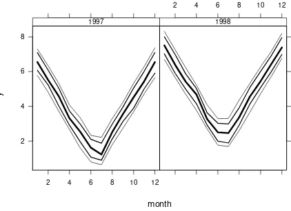
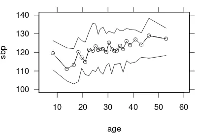
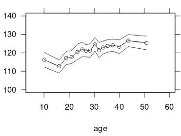
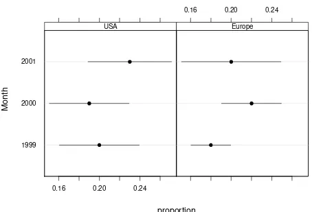
14.7.8 Error Bars and Bands . . . 139
14.7.9 Summary of Functions for Aggregating Data for Plotting . . . 152
15 Nonparametric Trend Lines 155 16 Reproducible Analysis, File and Script Management 158 16.1 File Management . . . 158
16.2 Script Management and Reproducible Analyses . . . 159
16.3 Reproducible Research . . . 162
Chapter 1
Overview of Computer Languages and
User Interfaces
1.1 Types of Products
·
Operating systems: Windows, Unix, Linux, MacOS·
Applications: Word, Excel, S-PLUS·
Commercial systems (Microsoft Windows and Office, S-PLUS, SAS, SPSS,Mac)
– Code, bug list secret
– Expensive unless your institution has a site license
– Upgrades increase cost even though don’t always add useful features
·
Free open-source systems (Linux, LATEX, StarOffice, R)– Revolution in software availability and function from the open source
CHAPTER 1. OVERVIEW OF COMPUTER LANGUAGES AND USER INTERFACES 3
movement
– Acceptance of free open-source APACHE Web Server by the commercial world and maturity of Linux has spearheaded this movementa
– Can see all code, change it, learn from it
– Quality generally quite good
– More rapid updates
– No one obligated to assist users but most products have an active and helpful user news group
– Lacks some bells and whistles such as extensive GUI
1.2 User Interfaces
·
Graphical (GUI, mouse, menus)– Easier to learn
– Less flexible
– Becomes repetitive when tasks repeated
– Hard to reproduce results
·
Command languages– Harder to learn
CHAPTER 1. OVERVIEW OF COMPUTER LANGUAGES AND USER INTERFACES 4
– More flexible and powerful
– Can save commands in scripts to replay when data updated or corrected, or to do similar analyses
– Can write generic commands (macros, functions) to make it easy to run different analyses that have same structure
1.3 Command Languages
·
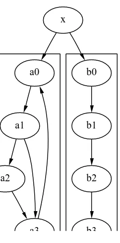
Specific purpose (e.g., draw a tree diagram, HTML)– Example: graphviz from www.research.att.com/sw/tools/
– dot program for drawing directed graphs (Emden Gansner, AT&T Re-search)
– Example code (in file clust1.dot):
digraph G {
subgraph cluster_c0 {a0 -> a1 -> a2 -> a3;} subgraph cluster_c1 {b0 -> b1 -> b2 -> b3;} x -> a0;
x -> b0; a1 -> a3; a3 -> a0; }
– Program run with the following DOS/Unix/Linux command line to produce PostScript graphic file clust1.ps
CHAPTER 1. OVERVIEW OF COMPUTER LANGUAGES AND USER INTERFACES 5
a0
a1
a2
a3
b0
b1
b2
b3 x
Figure 1.1:A directed graph produced by thedotprogram from the graphvizpackage.
See Section 2.1.2 for an example in which LATEX is used to draw a dia-gram.
·
Other specific-purpose languages include HTML, TEX, LATEX for web presen-tation or typesetting·
General purpose (C, C++, Python, Perl, Fortran, Java, S, Basic)– Compiled into machine code for fastest execution ∗ C, C++, Fortran
– Interpreted - run each statement as it’s encountered
∗ Allows executing statement by statement, selective execution of parts of code, very fast bug correction
∗ Examples: Perl, Python, Java, S, Basic
CHAPTER 1. OVERVIEW OF COMPUTER LANGUAGES AND USER INTERFACES 6
– Procedural: SAS
DATA new; SET old; htcm=htinches*2.54; PROC means; VAR htcm;
– Functional: Fortran, C, C++, Python, Perl, Java, S, Basic
2.54*mean(htinches) mean(htinches*2.54)
round(quantile((2*diastolic.bp+systolic.bp)/3))
·
Common Functions:Algebraic Form Computer Language
|x| abs(x)
ln x log(x)
ex exp(x)
√
x sqrt(x)
min(x1, x2, x3) min(x1,x2,x3) or min(x), x a vector
1.4 How to Learn Functional Languages
·
Learn the syntax, especially how arguments (parameters, options) are passed to functions·
Finding the right function for the job is the most difficult task·
Find functions by key words or phrases– Search S-PLUS and R functions: http://hesweb1.med.virginia.edu/ biostat/s/splus.htmlb
CHAPTER 1. OVERVIEW OF COMPUTER LANGUAGES AND USER INTERFACES 7
– Search S-PLUS functions by keywords: Contents button in Help GUI for S-PLUS Language
·
S Cheatsheet1.5 Types of Variables
·
integer·
floating point (scientific notation, e.g. 1.2e5 = 1.2×10⁵)– single precision (7 significant digits)
– double precision (15 digits)
·
character string, e.g. ‘Jim’·
categorical (“choice”), e.g., 1=good 2=better 3=best·
logical: TRUE, FALSE, T, F, 1, 0·
missing values: blank, ?, NA, .1.6 Complex Data Types
·
vector·
matrix: r ×cCHAPTER 1. OVERVIEW OF COMPUTER LANGUAGES AND USER INTERFACES 8
·
irregular structure (“list” or “tree”) e.g. states having variable number of coun-ties having varying number of cicoun-ties, data = population of city in 2000, popu-lation in 1990.1.7 Variables
·
Name of variable can be more than one letter; rules for names depend on language being used, e.g. age.yrs, X2, cholesterol, Age; may be case-sensitive·
Depending on language, variable name may stand for only one value of the variable at a time or it may stand for complex objects such as vectors, matri-ces, lists·
Variables vs. literals: ‘Jim’ is a particular value. Jim might be a variable containing a series of values.·
Examplessex <- ’female’ x <- 7+2
age.yrs <- age.days / 365.25
1.8 Types of User Files
·
Text — documents, simple data, commandsc·
Binary — Word documents, pdf files, datasetsCHAPTER 1. OVERVIEW OF COMPUTER LANGUAGES AND USER INTERFACES 9
Chapter 2
L
A
TEX
2.1 The Language
·
Text processing markup language by Leslie Lamport based on Knuth’s TEX language·
Used for compiling reports, books, articles·
Handles all details (microjustification, etc.) and is wonderful for math, chem-istry, and other symbols·
Interpreted command language·
Input is plain ASCII text, not binary, so can edit with any editora·
Example 1: Article style using enumerated list (auto-numbered); this is the “Bare bones plain LATEX example” at biostat.virginia.edu/latexaEditors such asEmacshave special modes to make editing LATEX code easier, and near-WYSIWYG systems such astexmacs, lyx, and
Scientific Wordtake this idea further.
CHAPTER 2. LATEX 11
\documentclass{article} % or report, book, ... \begin{document}
\title{Project 3}
\author{Jane Q. Public}
\date{\today} % or \date{2Jan01} for example
\maketitle % the \thanks line following is optional
\thanks{I neither gave nor received help on this project --- J.Q.P.} \begin{enumerate}
\item My answer to this question is unclear. \item Problem two was harder than problem 1.
The more I thought about it the less I knew.
\item % skip third problem
\item % stuff for 4th problem
\end{enumerate} \end{document}
To use bullet items substitute itemizefor enumerate
·
Here is an example where \section commands are used to automatically number (and optionally title) sections of the report.\documentclass{article} % or report, book, ... \begin{document}
\title{Project 3}
\author{Jane Q. Public}
\date{\today} % or \date{2Jan01} for example \maketitle
\section{} % Section 1, no title \section{Second Part}
My answer to this question is unclear. \section{Third Part}
CHAPTER 2. LATEX 12
·
To use Greek letters or other math symbols, go into math mode– Use $ $ within a line:
The result was $\tau=0.34$ and $R^{2}=0.65$, with $\alpha\geq 0.1$. Compare with $\frac{\gamma}{\gamma+\sqrt{\delta}}$.
– Or set off equations:
\begin{equation}
f(\gamma) = \sin^{-1}(\gamma) \end{equation}
The result is
f(γ) = sin−1(γ) (2.1) Note that \sin is special to LATEX, preventing sin from being italicized.
·
Make sure that any characters that are special to LATEX are “escaped” by prefixing them with\. For example, to print& % $ or #as regular characters change them to \& \% \$ \# in LATEX. If you leave% alone it will serve as the comment character for LATEX, causing the text to the right of it not to print.·
Make sure that any characters that LATEX needs to see only in math mode are somewhere surrounded by $ $. This pertains especially to < > _ ^if by the latter two you mean subscript and superscript. For example, replace R^2with $R^2$, a < 10 with $a < 10$, b > 10 with $b > 10$. For <= and >= use
\leq and \gte but with the whole expression surrounded by $ $.
CHAPTER 2. LATEX 13
$\beta_{1}$ is the coefficient of $X_{1}$; $F_{1,11}=1.2$.
results in
β1 is the cofficient of X1; F1,11 = 1.2.
·
Online help resources at biostat.virginia.edu/latex/2.1.1 Commonly Used LATEX Commands
Typed by User Result
\textbf{this} thisis boldface
\emph{this} thisis emphasized
$whatever$ Typesetwhateverin math mode
$\chi \tau \gamma \sigma \alpha$ χτ γσα
$\hat{Y} \neq 2 \times X\hat{\beta}$ Yˆ 6= 2×Xβˆ
$a \leq X \leq b, W < c, Z \geq a$ a≤X≤b, W < c, Z≥a
$\chi^2$ χ2
$X^{i+j}$ Xi+jto control which text is superscripted
$X_3$ X3subscript only one letter/number
$X_{i+1}$ Xi+1control what is subscripted
$\bar{X} = \sum_{i=1}^{n} X_{i}$ X¯=Pni=1Xi
\$100 $100 use $ without meaning math mode
\& \% \# \{ \} & % #{ }other special character escapes
\begin{enumerate} ... \end{enumerate} sequentially numbered list
\begin{itemize} ... \end{itemize} bullet list
\item text. . . entries for numbered or bullet items
~ force a blank character
\\ force a new line
\newpage force a new page
\section{text} start a new section, with title
2.1.2 Using LATEX andPSTricksfor Drawing Diagrams
·
Section 1.3 showed how a powerful standalone command languagegraphvizcan produce complex diagrams
CHAPTER 2. LATEX 14
·
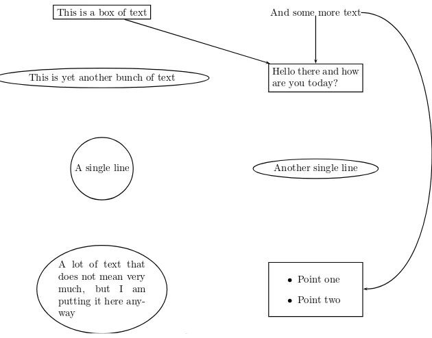
LATEX can be faster to use than drawing programs in many cases, with easier alignment of elements of a diagram, by thinking of the diagram as a matrix·
Example: The PSTricksLATEX package\usepackage{pstricks,pst-node}
% Define shorthand for a 20 character-wide centered-text parbox % This automatically formats multi-line boxes of text
\newcommand{\pb}[1]{\parbox[c]{20ex}{#1}} \centerline{\begin{psmatrix}
[name=A]\psframebox{This is a box of text} & [name=C]And some more text \\
\psovalbox{This is yet another bunch of text} &
[name=B]\psframebox{\pb{Hello there and how are you today?}} \\ \pscirclebox{A single line} &
\psovalbox{Another single line} \\
\psovalbox{\pb{A lot of text that does not mean very much, but I am putting it here anyway}} &
[name=E]\psframebox{\pb{
2.1.3 Benefits of LATEX for Statistical Reports
·
Automatic symbolic cross-referencingCHAPTER 2. LATEX 15
This is a box of text And some more text
This is yet another bunch of text Hello there and how are you today?
A single line Another single line
A lot of text that
Figure 2.1:A diagram produced byPSTricks
The theory behind this project can be summarized in the equation \begin{equation}
As seen in Section \ref{results}, Equation \ref{mc2} has
far-reaching implications. Figure \ref{myfigure} shows an example.
·
The\input{filename}and\includegraphics{filename}commands in LATEX can insert tables and graphs created by statistical programs.·
Adobe PostScript format is recommended for creating graphics files; LATEX renders these much better than Word renders Microsoft format graphicsre-CHAPTER 2. LATEX 16
computed) using latest versions of tables and graphs
·
There are functions in S-PLUS and R for automatically creating LATEX codefor complex tables
·
There is an option to make all references within the document clickable hy-perlinks in the final pdf file; these can be driven by automatically created tables of contents, figures, and tables, which is ideal for navigating long sta-tistical reportsb·
Excellent facility for handling bibliographic database and citing references in various styles·
Typical sequence:– Run S-PLUS to create or recreate tables and graphics files
– Run the latex system command on the LATEX master document to com-pile it
– Print the result or create a pdf file from it
– No manual operations such as menu selections for importing files into a Word document
·
Can construct batch programs for executing dataset operations, statistical analysis, and report building to make report reproducible when any compo-nent data change·
Seehesweb1.med.virginia.edu/biostat/s/doc/summary.pdffor a detailed how-to documentCHAPTER 2. LATEX 17
2.2 Biostatistics LATEX Web Server
·
You can install LATEX yourself but requires some effort and requires 100MB of disk space·
Can execute LATEX on a Linux server that has all the tools installed, including Ghostscript to convert to Adobe Acrobat Portable Document Format (PDF), a nearly-universal format for transmitting electronic documents·
The server can accept S-PLUS output with text to be sent to LATEX specifiedas S-PLUScomment lines. The server runs a reformatting program to create
the LATEX source code for a report.
·
Access the server at biostat.virginia.edu/latex or through the course web page·
In-class exercise:– Right click on the “Bare bones LATEX example” on the latex web page and save it to a temporary directory (in Wilson 308 a good area to use is \temp on C:) under any name you wishc
– Click on the link to the server and hit Browse to find the file you saved. Right click on this file to rename it to have a suffix of .tex. Get under
Browse again to select this file to upload it for processing.
NOTE: For all LATEX applications after this exercise and after Homework 1, you willnotneed to rename the file to upload to have a suffix of.tex. You only need to use this suffix to tell the server that you have a plain LATEX file. Ordinarily you will be uploading S-PLUS output, which can have any
file extension other than .tex.
– When LATEX compilation finishes, left click on the resultingpdf file to view it
CHAPTER 2. LATEX 18
– Right click on the pdf file and save it to a temporary area , then invoke
Chapter 3
Introduction to S
3.1 Statistical Languages and Packages
·
Procedure-oriented statistical packages– SAS, SPSS
– Lack of good interactive graphics
– Difficult to implement new methods
– Closed source — sometimes can’t find out how calculations done
·
Statistical language– S — object oriented
– Perl Data Language, MATLAB, Gauss
– Interactive graphics
CHAPTER 3. INTRODUCTION TO S 20
– Easy to implement new methods and distribute to others
– An open source version of S exists: R
3.2 Why S?
AH 1.1
·
S: a language for interactive data analysis and graphics·
Early on S was planned to be extendible– Users write new functions in the S language, same as developers
– Documentation for adding functions to the system is excellent
– User-added functions are invoked in same way as built-ins
– Users can create their own data types and add attributes such as com-ments to any piece of data in S
– Most users adding to a procedural system such as SAS write in a lan-guage (SAS macro or IML lanlan-guage) not used by SAS developers
– Very hard to write new SAS procedures
CHAPTER 3. INTRODUCTION TO S 21
·
Unlike macros, language is “live”, i.e., connected to the data while com-mands are runningif(is.category(x) | is.character(x) |
(is.numeric(x) & length(unique(x)) < 20)) table(x) else quantile(x)
Computes quantiles of a variable x if x is numeric and fairly continuous (at least 20 unique values), frequency tabulation otherwise
·
Object orientation means fewer commands to learn·
Second-order analyses easy; e.g. repeat a multi-step analysis multiple times perturbing the data slightly to see if results are unstable·
Best scientific graphics availableSAS graphics are ugly, inflexible, have poor defaults, difficult to program
3.3 History and Background of S-PLUS
KO pp. 1-4
·
S language developed at AT&T–Bell Labs, where C and UNIX were devel-oped·
Initial version 1976·
Usage increased rapidly after John Tukey’s book on exploratory data analy-sis published·
S-PLUS a commercial version of S, began 1987, popularity increaseddra-matically after 1990
CHAPTER 3. INTRODUCTION TO S 22
·
Provided and supported by Insightful Corporation (formally MathSoft)·
GUI, many formats supported for data import/export and graphics export (including Powerpoint and Windows metafiles)·
UVa has the most comprehensive site license available for S-PLUS3.4 R
AH 1.1.1
·
Statisticians around the world started developing R in early 1990s as an open source alternative to S-PLUS, partly to have a system on open sourceLinux which at the time was not supported by S-PLUS
·
Based on the same language used in S-PLUS 2000 with some minorexcep-tions
·
Well documented, easy to download and install from Internet; easy to update add-on libraries (“packages”) from Internet interactively·
Unlike S-PLUS can run on Macs·
No GUI on most platforms; rudimentary one on Windows·
Fewer data import/export capabilities than S-PLUS·
No explicit Powerpoint export capability·
Keep R in mind if your workplace does not wish to buy S-PLUS after youCHAPTER 3. INTRODUCTION TO S 23
·
Harrell’s S-PLUS libraries have been ported to R·
R’s web page is www.r-project.org3.5 Starting and Using S-PLUS on Windows
3.5.1 Starting S-PLUS
AH 1.2.2, KO 2.2
·
Lab computers: Run ... Program Files or desktop icon; may have to put S data objects in a public areaa·
On your own computer: make a desktop shortcut or better make a project directory and make a shortcut to splus.exefrom that project area·
If you put a shortcut to S-PLUS from your project area, carefully follow stepsin A&H 1.2.2 for modifying the shortcut properties to point to the project area for storing data and scripts instead of using the central system area
3.5.2 Command Window
·
Good for initial learning - results appear under your command·
Use ↑and ↓ keys to replay previously entered commands·
Use End key to go to end of line, Home key to go to start of line·
To exit S-PLUS enter the command q() or use File ... ExitCHAPTER 3. INTRODUCTION TO S 24
3.5.3 Script Window
KO 2.16, AH 1.5, UG 8
·
Recommended when the task involves more than a few commands·
Script editor has nice features·
Can fit F10 to submit all commands in script editor window (if none high-lighted) or just the highlighted ones·
Depending on system option settings, output from those commands will be at the bottom of the script window·
Can use a system option to divert output to a cumulative Report WindowChapter 4
S Language
KO 3, AH 1.4, UG 9, PG 1
4.1 General Rules
KO 1.3
·
Prompt for commands in command window: >·
Continuation prompt when command incomplete: +·
Neither of these ever typed by user·
Command can be any length·
If you want to break a long command into multiple lines for readability, make sure S-PLUS knows that more is to come by making the current lineincom-plete
– Example: end the line with one of the three characters ({,
·
Multiple commands may appear on one line if separated by ;CHAPTER 4. S LANGUAGE 26
·
Text after # considered comment and ignored·
Spaces and tabs in commands are ignored except when in quotes·
Doesn’t matter if use single or double quotes as long as– you use the same type of quote to close as you used to open
– no quote of same type within a string being quoted (in that case quote with the unused character)
·
On Windows systems (but not Linux/UNIX), file names in quotes are notcase-sensitive
·
Indent most continuation lines for readability·
In the Command Window you can use the Home and End keys to move to the start or end of a line to make corrections. You can submit the command for execution by hitting Enter without moving the pointer to the end of the line.·
Use ↑ and ↓ keys to replay previously entered commands; these may be modified and then submitted·
Use the Command History window to resubmit blocks of lines at one time4.2 Types of Basic Data in S
·
numeric– integer
CHAPTER 4. S LANGUAGE 27
∗ default: double precision—15 sig. digits
∗ single precision—7 digits of precision a
·
character string·
logical·
list: collection of several objects of any types·
function4.3 S As a Calculator: Arithmetic Expressions
·
Try examples such as the following17 # nothing to do but print 17
17/2 # division
1+1 # evaluated left to right
1+2*3+10 # multiplication (*) takes priority over addition 1+2^3 # exponentiation (2 to the 3rd power) done first 1+2^3*7 # exponentiation, then multiplication, then addition sqrt(4) # square root function
1+2*sqrt(9*9) # everything inside () finished first, then sqrt, *, +
3+ # S will wait for more
4 # 7
·
Note that when you submit a command to S that is not inside { } the result of the command will be printed automatically·
Use ( ) to group expressions so that order of evaluation is obvious2*(3+4) 2*(3+4)^2
CHAPTER 4. S LANGUAGE 28
4.4 Assignment Operator
·
Used to create a variable or other S object·
Variable names may contain the symbols a-z,A-Z,0-9 and . but may notstart with a number AH 2.1
– They may not contain the underscore character or a blank
– When importing data containing illegal field names, S will often convert these to legal S names but it’s best to change these names to legal S names yourself during the import
·
Names are case-sensitive·
Recommended that you surround the assignment operator (<-) by spaces·
Examples:x ← 4
x # prints value of x, 4
sqrt(x)-3/2 x ← x*2 x
1/x x-1
y ← (x+11*2)/2 y
description ← ’This analysis is revealing’ description
CHAPTER 4. S LANGUAGE 29
4.5 Two Frequently Used Functions
·
Typeprint(expression)orprint(variablename)to print the result ofexpressionor contents of variablename
– This is only necessary if you want to control formatting of printing or are printing from within a function or other expression enclosed by { }
·
Type rm(x), remove(’x’), rm(x,y), remove(c(’x’,’y’)) to remove ob-ject x or objects x and y from storage4.6 Making Vectors
AH 2.4
·
The S function named c combines elements into a vectorz ← c(’cat’,’dog’) # character string vector
z # note [1] in output - refers to element 1
c(description, description) c(1,x)
c(1,x)*2 # arithmetic on vector does same thing many times 2*c(1,x)
c(1,2,7) x ← c(1,2,7)
length(x) # returns number of scalar elements x/2
c(c(1,4),c(2,5))
·
When the values are from a systematic sequence you can save codingrep(2.1, 30) rep(’garbage’,5) rep(c(1,3),2)
1:10 # generates a sequence with increment 1.0
10:1 # decrement 1
seq(1,10) # same thing
seq(1,10,1) # same thing
seq(1,10,by=1) # same thing
seq(1,10,by=2) # increments by 2 but not to exceed 10 seq(1,10,by=-2) # illegal increment
CHAPTER 4. S LANGUAGE 30
seq(5,1,by=-1)
4.7 Logical Values
·
Values of TRUE or FALSE (abbreviated T,F)·
Treat TRUE like 1, FALSE like 0·
Logical negation operator: !x ← T # or TRUE
!(2 > 3) # watch out on some systems: ! as first character # can mean ’send rest of line to operating system’ # to be safe can do (!(2 > 3))
·
Logical union (or), intersection (and): | & F | F·
To compute a TRUE,FALSE on the basis of an equality use == x ← 6CHAPTER 4. S LANGUAGE 31
·
A missing numeric or character value may begin as a blank in a spreadsheet·
Symbol for missing numeric value in S: NAx ← NA
·
To sense that a value is missing never use ==, use the is.na function:is.na(x)
x.present ← !is.na(x) x.present
·
Unlike SAS, S determines inequalities correctly when NAs presentx < 2
CHAPTER 4. S LANGUAGE 32
4.9 Summary: S Cheatsheet
Compiled by Barry W. Brownb Department of Biomathematics
University of Texas M. D. Anderson Cancer Center Houston, TX 77030
CHAPTER 4. S LANGUAGE 33
%% Remainder or modulo operator
CHAPTER 4. S LANGUAGE 34
> Greater-than
>= Greater-than-or-equal-to
4.9.4 Logical Operators
! Not
| Or (Use with arrays or matrices)
|| Shortcut Or (Don’t use with arrays or matrices)
& And (Use with arrays or matrices)
&& Shortcut And (Don’t use with arrays or matrices)
Above “shortcut” means that if the condition is not satisfied, the remaining parts of the expression are not even evaluated. This is very useful if these parts don’t even make sense then, or are slow to execute.
4.9.5 Subscripts
[ ] Vector subscript
[[ ]] list subscript - can only identify a single element
$ Named component selection from a list
Subscript Forms
logical extracts or selects T component
positive numbers extracts or selects specified indices
negative numbers deletes specified indices
NA or out of range extends dimensions gives value NA
4.9.6 Sequence and Repetition
seq (from, to, by, length, along)
also : as in 1:10
CHAPTER 4. S LANGUAGE 35
4.9.7 Arithmetic Operators and Functions
abs(x)
Can be used in as.<type> and is.<type> and <type>(length)
CHAPTER 4. S LANGUAGE 36
sink( ) restores output to screen
Write and Read Objects
dput(x, file) writes out object in S notation dget(file)
write(t(matrix),file,ncol=ncol(matrix),append=FALSE)
data.dump(objnames, file=’filename’) objnames may be ’obj name’ or c(’name1’,’name2’,...) data.restore(’filename’)
Make Things (Including Help) Available or Unavailable
assign("name", value, frame, where)
attach(file, pos=2) detach(2)
library( )
library(help=section)
library(section, first=TRUE) make library’s functions take precedence
CHAPTER 4. S LANGUAGE 37
p<dist>(x,<parameters>) cumulative distn fn to x
q<dist>(p,<parameters>) inverse cdf
r<dist>(n,<parameters>) generates n random numbers from distn
<dist> Distribution Parameters Defaults beta beta shape1, shape2 , -cauchy Cauchy loc, scale 0, 1 chisq chi-square df -exp exponential -
-f F df1, df2 ,
-gamma Gamma shape -lnorm log-normal mean, sd (of log) 0, 1 logis logistic loc, scale 0, 1 norm normal mean, sd 0, 1 stab stable index, skew -, 0 t Student’s t df -unif uniform min, max 0, 1
4.9.12 Plotting
Starting and Stopping Plotting
CHAPTER 4. S LANGUAGE 38
new=<logical> T forces addition to current plot
sub=’bottom title’
type=’<l|p|b|n>’ Line, points, both, none
lty=n Line type
barplot(height, width, names, space=.2, inside=TRUE, beside=FALSE, horiz=FALSE, legend, angle, density, col, blocks=TRUE)
boxplot(..., range, width, varwidth=FALSE, notch=FALSE, names, plot=TRUE)
hist(x, nclass, breaks, plot=TRUE, angle, density, col, inside)
Two-Dimension Plots
lines(x, y, type="l") points(x, y, type="p"))
CHAPTER 4. S LANGUAGE 39
matlines(x, y, type="l", lty=1:5, pch=, col=1:4)
plot(x, y, type="p", log="")
abline(coef) abline(a, b) abline(reg) abline(h=) abline(v=)
qqplot(x, y, plot=TRUE)
qqnorm(x, datax=FALSE, plot=TRUE)
Three-Dimension Plots
contour(x, y, z, v, nint=5, add=FALSE, labex)
interp(x, y, z, xo, yo, ncp=0, extrap=FALSE)
persp(z, eye=c(-6,-8,5), ar=1)
Multiple Plots Per Page (Example)
par(mfrow=(nrow, ncol), oma=c(0, 0, 4, 0)) mtext(side=3, line=0, cex=2, outer=T,
Chapter 5
Objects, Getting Help, Functions,
Subsetting, Attributes, and Libraries
5.1 Objects—General
AH 2.1, KO p. 70
·
Everything in S is an object·
Work on objects by applying functions to them·
Usually an object is ultimately committed to a disk file with the same name as the S objecta5.2 Functions
KO 4.2, AH 2.3
5.2.1 Getting Help
AH 2.2, KO 3.1.2
·
To find out how to use a functionaIn Windows, disk file names do not correspond to object names if the object name is longer than 8 characters.
CHAPTER 5. OBJECTS, GETTING HELP, FUNCTIONS, SUBSETTING, ATTRIBUTES, AND LIBRARIES 41
·
At command line (or submit run using F10 if using Script window) type?functionname if you know its name
·
May want to look at examples first then work backwards to details·
Specifications and data are passed to functions as arguments·
If you know what a function does and just need to know the names and order of its arguments type args(functionname)This also shows the default values of the arguments that are used when you do not provide a value for the function.
Note: When the default value for an argument is a vector like
c(value1,value2,value3), and the argument really takes a scalar value, the default value for the argument is value1 and the other values are the only other possible values for that argument.
·
Sometimes you need to find out exactly what a function does. You can often print its full definition by running the command functionname, which runsprint(functionname).
·
For Windows S-PLUS there are good ways to find which function to use byusing the Language Reference submenu on the Help menu:
– tell you which functions contain a word or phrase you specify anywhere in its help file, and let you click on one of those functions to see its help file if you click on Search
– put of a list of keywords around which functions are organized and let you click on a keyword to list all the functions related to that area if you click on Contents; then you can go to help files for individual functions AH 2.2
CHAPTER 5. OBJECTS, GETTING HELP, FUNCTIONS, SUBSETTING, ATTRIBUTES, AND LIBRARIES 42
5.2.2 Using Functions
·
An S command line can look likefunctionname(argument1, argument2, argument3)
which will run function functionname on the values given by the arguments
argument1, argument2, argument2 and will print the result returned by the function
·
Arguments are frequently called parameters, especially when you are look-ing inside the body of a function definition·
Some functions which only do things such as make a plot in a graphics window or to a graphics device do not have any results printed·
Often functions are invoked using a format such asfunctionname(major.data.object, otherarguments)
whereotherargumentsare variables or constants whose values tell the func-tion how to operate on the main data given by major.data.object or they tell the function exactly what the function should compute
·
We often think of such other arguments as options·
For many functions, we pass the first argument by position, which means that the function will know what to do with that object by virtue of it being the first argument·
This first argument is often a variable to analyze·
Other arguments may also be specified by position, but functions have to give their own internal names for arguments and we can match arguments to values we defined by specifying argument names in the formCHAPTER 5. OBJECTS, GETTING HELP, FUNCTIONS, SUBSETTING, ATTRIBUTES, AND LIBRARIES 43
·
Don’t need to give values to all arguments to a function because some may not be needed for a particular analysis and others may have default values we like·
Passing arguments by name does away with need to remember order of arguments·
Example: mean has arguments x, trim, na.rm:> args(mean)
function(x, trim = 0, na.rm = F)
– 1st argument: x (vector to analyze), no default value
– 2nd: trim—amount of trimming of outer values to use default is zero (compute ordinary mean)
– 3rd: na.rm—defaults to F (false), which means that NAs are not automat-ically removed from x before computing the mean; if NAs are present, the resulting mean would be NA
Set na.rm=Tto make the mean function removeNAs before computing the mean
This results in the mean of all non-missing values
·
To compute the mean of age while ignoring NAs, we could use the S com-mand mean(age, , T)·
Interpret as passing T as the value of the 3rd argument na.rmCHAPTER 5. OBJECTS, GETTING HELP, FUNCTIONS, SUBSETTING, ATTRIBUTES, AND LIBRARIES 44
5.3 Subsetting Vectors
AH 2.4.3, KO 3.2
·
[ ] after an object name subsets the object·
Different objects use different subsetting methods– For a tree (hierarchical list object) a subset may be a subtree
– For a vector it may be a subvector
– For a matrix it may be a submatrix or a row or column
·
To subset to an individual element use e.g.x2 ← x[2] # retrieve the second element of vector x
·
To get a subset that is more than one element:x.small ← x[3:5] # get x[3], x[4], x[5] and put in x.small y ← x[c(2,5)] # get x[2] and x[5]
z ← x[-3] # get all but x[3]
z ← x[-c(2,5)] # get all but x[2] and x[5]
·
x[3:5] uses an index vector 3:5 to select elements·
Can also use logical vectors to select elements– T means to select element
– F means to ignore element
CHAPTER 5. OBJECTS, GETTING HELP, FUNCTIONS, SUBSETTING, ATTRIBUTES, AND LIBRARIES 45
·
Very often we use logical expressions to get subvectors to analyze:> sex ← c(’m’,’f’,’m’,’m’) > x ← 1:4
> x[sex==’m’]
[1] 1 3 4
·
Other common examples are x[!is.na(x)] and x[y>3 & w < 2]5.4 Matrices, Lists, Data Frames
KO 4.1, AH 2.5, PG 3
5.4.1 Matrices
AH 2.5.1
·
Two-dimensional arrays—rows and columns·
All elements of same type (numeric or character)·
Built by using the matrix function or by combining vectors assuming they represent rows (rbind()) or columns (cbind()) of the new matrix·
One way to subset matrices is to specify either vectors of row and column numbers (or both)·
Can define row and column names; dimnames contain both of these·
When a matrix has dimnames you can also subset the matrix using vectors containing row and/or column names·
Example:CHAPTER 5. OBJECTS, GETTING HELP, FUNCTIONS, SUBSETTING, ATTRIBUTES, AND LIBRARIES 46
> x ← cbind(a,b) # row names not defined > x
a b
[1,] 1 4
[2,] 2 5
[3,] 3 6
> x[2:3,]
a b
[1,] 2 5
[2,] 3 6
> x[,2]
[1] 4 5 6
> x[,’b’]
[1] 4 5 6
·
The apply function will compute arbitrary statistics over either the rows or the columns of the matrix5.4.2 Lists
AH 2.5.2
·
Lists are hierarchical collections of objects with no symmetry requirement·
Can be a collection of vectors of different lengths·
Often a collection of scalars and vectors or matrices·
Lists are incredibly flexible—can contain other lists·
Good way to store a treeCHAPTER 5. OBJECTS, GETTING HELP, FUNCTIONS, SUBSETTING, ATTRIBUTES, AND LIBRARIES 47
having the same length
·
A list is created using the list function.The names of its arguments specify the names of the elements of the list.
·
See AH 2.5.2 for an example showing the flexibility of lists:us ← list(Alabama=list(counties=c(Autauga=40061,Baldwin=123023,...), pop=4273084,capital=’Montgomery’),
Alaska=list(counties=c(’Aleutians East’=2305,...), pop=602545,capital=’Juneau’),
...)
us$Alabama # retrieve all info about Alabama
us$Alabama$counties # retrieve all county names and pop. us$Alabama$counties[1:5] # first 5 counties
us$Alabama$capital # scalar character value us[c(’Alabama’,’Alaska’)] # sub list with only 2 states Ak ← us$Alaska # new list with only Alaska data
Ak$counties # fetch counties for Alaska
In the definition of the uslist, thecountiesvectors werenamed vectors. The values of these vectors are the county populations but these will be labeled, and the population for a given county may be obtained using the county name in addition to using the county position (if known). For example:
us$Alabama$counties[’Baldwin’]
retrieves the population of Baldwin county in Alabama.
·
One of the most common uses of lists is to hold the results of fitting a regres-sion model. These results may consist of a vector of regresregres-sion coefficients, a matrix of variances and covariances for these coefficients, and scalars such as R2.5.4.3 Data Frames
AH 2.5.3
CHAPTER 5. OBJECTS, GETTING HELP, FUNCTIONS, SUBSETTING, ATTRIBUTES, AND LIBRARIES 48
·
A list made up of one or more vectors of the same length·
Unlike a matrix, these vectors may have differing types·
Unlike a generic list, data frames have special subscripting methods ([]methods) that allows one to easily subset allof its component vectors
·
Data frames are created when datasets are imported, or using thedata.framefunction:
mydata ← data.frame(age=c(10,20,30), sex=c(’female’,’male’,’male’))
This is the same as doing
mydata ← list(age=c(10,20,30), sex=c(’female’,’male’,’male’))
except that a data frame has attributes that lists do not have:
dim : a 2-element vector containing number of rows and columnsb
rownames : a character vector containing row names (often this is a subject ID)
class : the class of a data frame is ’data.frame’; this insures that spe-cial methods (print.data.frame and [.data.frame respectively) will be used to print and to subset the object
– print(mydata) invokes print.data.frame(mydata) to print the data in columns
– [.data.frame] allows you to easily extract a sub-data frame by spec-ifying the rows and columns of interest
·
To specify the row.names to use when creating the data frame, tell a data import procedure to use a certain input column as the observation IDs, or do something likemydata ← data.frame(age=c(10,20,30), sex=c(’f’,’m’,’f’), row.names=c(’A1’,’A2’,’B20’))
CHAPTER 5. OBJECTS, GETTING HELP, FUNCTIONS, SUBSETTING, ATTRIBUTES, AND LIBRARIES 49
If row.names are not defined they will default to c(’1’,’2’,...). For the above mydata data frame you can extract subsets using these examples:
mydata$sex # get the sex variable (vector)
mydata[,’sex’] # same
mydata[,c(’age’,’sex’)] # new data frame, 2 variables, but same as old
mydata[1:2,] # new data frame, only 2 obs.
mydata[1:2,’age’] # new vector, 2 obs.
mydata[’A1’,] # new data frame, 1 obs., all vars. mydata[c(’A1’,’A2’),] # new data frame, 2 obs.
mydata[1:2,] # ditto
·
One subtle difference between data frames and lists: when creating data frames, character vectors such as sex are usually translated to S factorvariables
5.5 Attributes
AH 2.6
·
Extra information tagged onto an object·
Not the value of the object used in computation– matrices have dim and dimnames
– data frames have class, row.names, and names (the names of the vari-ables) and effectively have dim
– lists have names: names of major elements
– factors have levels and class
·
Attributes may be retrieved byCHAPTER 5. OBJECTS, GETTING HELP, FUNCTIONS, SUBSETTING, ATTRIBUTES, AND LIBRARIES 50
– attributes(objectname)$attributename
– extractor functions such as dim,names,class,row.names
·
If a vector is given element names, the vector has these stored in the namesattribute
> x ← c(Alabama=23, Ohio=12) > x
Alabama Ohio
23 12
> names(x)
[1] "Alabama" "Ohio"
·
Users may add their own attributes on the fly:> attr(age,’comment’) ← ’for children age was estimated’ > attr(age,’comment’)
[1] ’for children age was estimated’
·
class is a very special attribute that allows S to be object-oriented– Class of an object triggers methods to handle that object
– generic.function.name(object) will invoke
generic.function.name.class(object), whereclassis the object’s ma-jor class
– Subclasses are allowed and these will invoke specific methods with no special methods are present for handling major class
CHAPTER 5. OBJECTS, GETTING HELP, FUNCTIONS, SUBSETTING, ATTRIBUTES, AND LIBRARIES 51
·
Ex: class(mydata) may be ’data.frame’ class(mydata$sex) is’factor’5.6 Factor Variables
AH 2.6.1
·
Vectors of categorical data·
Most useful when there are many fewer categories than there are subjects·
Label for each category (“value labels”)·
Internally factors are stored as positive integers·
Factors created during data import, by data.frame function, or by using thefactor function:
> sex ← c(1,2,1) # original coding on source database > sex ← factor(sex, 1:2, c(’female’,’male’))
> class(sex)
> sex ← factor(sex, c(’f’,’m’), c(’female’,’male’)) > sex
CHAPTER 5. OBJECTS, GETTING HELP, FUNCTIONS, SUBSETTING, ATTRIBUTES, AND LIBRARIES 52
·
Note that data can originate as character or numeric·
If you always specify a 2nd argument to factor you will always make it clear how factor levels correspond to the original values·
In programming usually treat factor variable as a character string:age[sex==’female’] # get subvector of ages for females
age[sex!=’male’] # same thing
fem ← sex==’female’ # create new logical variable
females ← mydata[mydata$sex==’female’,] # females, all columns sexc ← as.character(sex) # force into character vector
·
The print.factor method for factors prints the formatted values, without quotes5.7 When to Quote Names
AH 2.7
·
Always quote character string constants (literals)·
Quote variable names when they are used to specify which variables to re-trieve from a list or data frame and $ is not used to do this·
Otherwise S will try to find variables whose names are the values of the object you specifiedCHAPTER 5. OBJECTS, GETTING HELP, FUNCTIONS, SUBSETTING, ATTRIBUTES, AND LIBRARIES 53
5.8 Hmisc Add-on Function Library
AH 2.9
·
Libraries (called packages in R)contain a bunch of related functions and all their online help files; may contain test datasets also·
S has several libraries builtin·
Users adding more than one function to S usually put the functions in an add-on library·
Huge number of add-on libraries available·
Hmisc library: variety of added functions for– data analysis and data reduction
– high-level graphics
– utilities
– sample size, power
– converting SAS datasets to S data frames
– imputing missing data
– advanced table making
– conversion of S objects to LATEX code
CHAPTER 5. OBJECTS, GETTING HELP, FUNCTIONS, SUBSETTING, ATTRIBUTES, AND LIBRARIES 54
·
Windows S-PLUS comes with Hmisc library builtin·
Get updates fromhesweb1.med.virginia.edu/biostat/s/Hmisc.htmlwhich also has a link to a page telling how to install the libraryc·
Installation on Windows systems just involves unzipping a file stored in a temporary disk file into the correct subdirectory in the area where S-PLUSisinstalled
·
Libraries are “attached” using the library function or the File ... Load Library menu·
Hmisc needs to override a few builtin S functions so it needs to be attached in the search list (which will be covered later) before the system functionsd·
The main function redefined by Hmisc is the subsetting function for factors,[.factor. [.factor in Hmisc by default will remove unused levels from a factor variable if the resulting subset did not use that levele
·
To make Hmisc automatically available every time S-PLUS is invoked, putthe following in the script or command window and run it:
.First ← function(...) { library(Hmisc,T)
invisible() }
·
.First is a user-defined function that is executed when S-PLUS starts froma project area whose Data directory contains the .First function
·
If you don’t set up .First or use the File ... Load Library menudur-cAt present no updates are available for S-PLUS6.
CHAPTER 5. OBJECTS, GETTING HELP, FUNCTIONS, SUBSETTING, ATTRIBUTES, AND LIBRARIES 55
ing the session you can make the functions in the library available using
library(Hmisc,T) in your program
·
On Windows platforms, Hmisc comes with a Microsoft Windows Help file that is easy to navigate·
To navigate the library typehelp(library=’Hmisc’)orlibrary(Hmisc,help=T)(but not in R) or click on the special menu created for Hmisc the first time
Chapter 6
Turning S Output into a L
A
TEX
Report
·
Used to typeset text in the bottom pane of the Script window or text saved from a Report window into a report in Adobe Acrobat Portable Document Format (pdf)·
The Report window is slightly preferred as it is cumulative (has all the com-mands and output for the whole sessiona and File ... Save as works when the Report window is active (unlike the bottom pane of the Scriptwindow).
·
To make output go to theReportwindow, select it after navigating theOptions ... Text Output Routingmenus·
If using a Report window do not save it as a binary .srp report file; save files as plain text, i.e., .txt is a good suffix·
S-PLUS has an annoying habit of moving some comment lines when writingto the Report window. When these comment lines contain text for LATEX to process (see later) this can be a real problem.
aIf you have to run sections of code more than once to succeed, you will need to delete unneeded input and output from theReport window.
CHAPTER 6. TURNING S OUTPUT INTO A LATEXPDFREPORT 57
·
Also, it is good practice to be able to run the S-PLUS script from scratch.Running a batch job will do this, once you have interactively debugged the script. Using the commands below will also prevent S-PLUSfrom
reposition-ing comment lines. Use Notepad to create a file called s.bat in your project area or in a folder in your system file path. s.bat should contain the following commands.
set SHOME=’’c:\Program Files\splus61’’ or wherever S-Plus is
set S_PROJ=c:\temp or wherever project folder is
set S_CWD=%S_PROJ%
’’c:\Program Files\splus61\cmd\sqpe’’ < %1.s > %1.txt replace .s with .ssc
This is a DOS batch file that when invoked with the DOS orRun ... Command
command ofs myfilewill run the scriptmyfile.s(ormyfile.sscdepending on the prefix used above) and create a report file myfile.txt. Running sqpe
rather than the regular splus.exe command runs S-PLUS without the GUI
and makes it run faster while using less RAM. If you storeds.bat on a floppy disk for use in the lab you can run it by typing the command a:\s myfile or
a:\s \projects\myproj\myfile, for example.
·
But his method does not print the S-PLUS commands in the .txt file; do make that happen put the following command at the top of the script:options(echo=T)
·
The server reformats S output such as the .txt file into LATEX code, running the LATEX compiler stored on the server to create a PostScript document, and running the Ghostscript command to convert the Postscript docu-ment to pdf·
Helps greatly with incorporating high quality graphics in a report (to be cov-ered later)CHAPTER 6. TURNING S OUTPUT INTO A LATEXPDFREPORT 58
S commands that carried this out) and interpretation of results (generally appearing after the S code in the .ssc file).
·
The server creates a LATEXarticle style document·
Always refer to the many documentation files on the server for more info·
When you upload a plain text ASCII file that does not have a suffix of .texto the biostatistics LATEX server, the server assumes that
– All text after # comprise LATEX code, sent to LATEX without change (except for the #@caption directive used in plotting (later))
These are comments to S and are ignored by S
– Your file does not contain LATEX preamble and postamble material; these are added automatically by the server
– Various commands are in certain formats when your program creates graphics (later)
– Any text not preceded by # is assumed to be either S commands or S output
∗ S output is included as-is in the report using a LATEXverbatim environ-ment
∗ S commands are parsed so that
· <-is converted to←by replacing it with a macro\Gets used by the
S.sty package that the server calls to typeset S code neatly
· { } are converted to \{ \} so they will be typeset to print as{ }
CHAPTER 6. TURNING S OUTPUT INTO A LATEXPDFREPORT 59
· S comments after # are printed in a smaller font by wrapping that text in a macro \scom{...text...}; it would be easy to define the
scom macro to typeset comments in different fonts or colors.
·
Lines beginning with # are sent to LATEX with the following changes– # symbol removed
– <= >= < > are changed to $\leq$ $\geq$ $<$ $>$ if the line does not already have two $ in it
·
As LATEX’s comment symbol is %, any text that you don’t want to typeset should be in an S comment line (# ...) and that text should be preceeded by %·
It is recommended that you include title and date information·
Most reports will have sections; homeworks will have sequentially numbered problems·
For the latter, use a LATEXenumerateenvironment with each problem starting with \item (or use \section{})6.1 Example S Output
Suppose you save the following into a file test.txt in your project directory.
CHAPTER 6. TURNING S OUTPUT INTO A LATEXPDFREPORT 60
##f
# This is an example report. Line 2 is # continued here.
> # This should be treated as if the > weren’t there, as
# S-Plus sometimes adds > in the bottom panel of a \texttt{Script} # window. Here we use math mode $x+y$.
x <- matrix(runif(9), nrow=3) # create a matrix # More text
if(1==2) { y <- 3 }
The temporary LATEX code produced by the server would be
\documentclass{article} \usepackage{graphicx} \usepackage{ccapt2}
\usepackage{S} % S style macros for typesetting S code \usepackage[bookmarks,pdfpagemode=UseOutlines]{hyperref} %For commands at the right of S-Plus code lines:
\newcommand{\scom}[1]{{\rm\scriptsize \# #1}}
... commands to set up for making simple tables (not shown) ... ... commands to set up for graphics (not shown) ...
\begin{document}
CHAPTER 6. TURNING S OUTPUT INTO A LATEXPDFREPORT 61
This is an example report. Line 2 is continued here.
This should be treated as if the $>$ weren’t there, as
S-Plus sometimes adds $>$ in the bottom panel of a \texttt{Script} window. Here we use math mode $x+y$.
\begin{Example}
x \Gets matrix(runif(9), nrow=3) \scom{create a matrix} \end{Example}
Note that a lone > was translated to math mode ($>$) Here is a typical example, starting the the S output file saved by the user.
#\title{Project 2}
#\author{Jane Q. Public}
#\date{\today} % or \date{2Jan01} for example #\maketitle
#\thanks{I neither gave nor received help on this project --- J.Q.P.} #\begin{enumerate}
#\item % first problem
#My approach to this problem involved ... x <- rnorm(1000)
#You can see a Gaussian shape in the histogram. #More conclusions.
#\item % skip second problem
#\item % third problem
#One can see that ... #\end{enumerate}
CHAPTER 6. TURNING S OUTPUT INTO A LATEXPDFREPORT 62 %For commands at the right of S-Plus code lines:
CHAPTER 6. TURNING S OUTPUT INTO A LATEXPDFREPORT 63
\date{\today} % or \date{2Jan01} for example \maketitle
\thanks{I neither gave nor received help on this project --- J.Q.P.} \begin{enumerate}
\item % first problem
My approach to this problem involved ... \begin{Example}
x \Gets rnorm(1000) \end{Example}
You can see a Gaussian shape in the histogram. More conclusions.
\item % skip second problem
\item % third problem
One can see that ... \end{enumerate}
\end{document}
6.2 Common Errors
·
Not putting things like R^2, x<y in math mode (but only inside S comment lines that become open LATEX code)·
Not escaping % $ & #by typing \% \$ \& \#when used in S comment lines to represent percent or dollars·
Not correcting S-PLUS’s reformatting of some comment lines. Often S-PLUSwill move a comment line to the end of the previous S command. This will run things together. Edit such lines by hitting Enterto move the # ... comment ... back to the next line where it belongs (this is not a problem if using the
sqpe batch file method).