Finite Difference Methods
in Financial Engineering
A Partial Differential Equation Approach
Finite Difference Methods
in Financial Engineering
A Partial Differential Equation Approach
Published by John Wiley & Sons Ltd, The Atrium, Southern Gate, Chichester, West Sussex PO19 8SQ, England
Telephone (+44) 1243 779777
Email (for orders and customer service enquiries): [email protected] Visit our Home Page on www.wiley.com
All Rights Reserved. No part of this publication may be reproduced, stored in a retrieval system or transmitted in any form or by any means, electronic, mechanical, photocopying, recording, scanning or otherwise, except under the terms of the Copyright, Designs and Patents Act 1988 or under the terms of a licence issued by the Copyright Licensing Agency Ltd, 90 Tottenham Court Road, London W1T 4LP, UK, without the permission in writing of the Publisher. Requests to the Publisher should be addressed to the Permissions Department, John Wiley & Sons Ltd, The Atrium, Southern Gate, Chichester, West Sussex PO19 8SQ, England, or emailed to [email protected], or faxed to (+44) 1243 770620.
Designations used by companies to distinguish their products are often claimed as trademarks. All brand names and product names used in this book are trade names, service marks, trademarks or registered trademarks of their respective owners. The Publisher is not associated with any product or vendor mentioned in this book.
This publication is designed to provide accurate and authoritative information in regard to the subject matter covered. It is sold on the understanding that the Publisher is not engaged in rendering professional services. If professional advice or other expert assistance is required, the services of a competent professional should be sought.
Other Wiley Editorial Offices
John Wiley & Sons Inc., 111 River Street, Hoboken, NJ 07030, USA Jossey-Bass, 989 Market Street, San Francisco, CA 94103-1741, USA Wiley-VCH Verlag GmbH, Boschstr. 12, D-69469 Weinheim, Germany
John Wiley & Sons Australia Ltd, 42 McDougall Street, Milton, Queensland 4064, Australia John Wiley & Sons (Asia) Pte Ltd, 2 Clementi Loop #02-01, Jin Xing Distripark, Singapore 129809 John Wiley & Sons Canada Ltd, 22 Worcester Road, Etobicoke, Ontario, Canada M9W 1L1 Wiley also publishes its books in a variety of electronic formats. Some content that appears in print may not be available in electronic books.
Library of Congress Cataloguing-in-Publication Data Duffy, Daniel J.
Finite difference methods in financial engineering : a partial differential equation approach / Daniel J. Duffy. p. cm.
ISBN-13: 978-0-470-85882-0 ISBN-10: 0-470-85882-6
1. Financial engineering—Mathematics. 2. Derivative securities—Prices—Mathematical models. 3. Finite differences. 4. Differential equations, Partial—Numerical solutions. I. Title.
HG176.7.D84 2006
332.01′51562—dc22 2006001397
British Library Cataloguing in Publication Data
A catalogue record for this book is available from the British Library ISBN 13 978-0-470-85882-0 (HB)
ISBN 10 0-470-85882-6 (HB)
Typeset in 10/12pt Times by TechBooks, New Delhi, India
Contents
0 Goals of this Book and Global Overview 1
0.1 What is this book? 1
0.2 Why has this book been written? 2
0.3 For whom is this book intended? 2
0.4 Why should I read this book? 2
0.5 The structure of this book 3
0.6 What this book does not cover 4
0.7 Contact, feedback and more information 4
PART I THE CONTINUOUS THEORY OF PARTIAL
DIFFERENTIAL EQUATIONS 5
1 An Introduction to Ordinary Differential Equations 7
1.1 Introduction and objectives 7
1.2 Two-point boundary value problem 8
1.2.1 Special kinds of boundary condition 8
1.3 Linear boundary value problems 9
1.4 Initial value problems 10
1.5 Some special cases 10
1.6 Summary and conclusions 11
2 An Introduction to Partial Differential Equations 13
2.1 Introduction and objectives 13
2.2 Partial differential equations 13
2.3 Specialisations 15
2.3.1 Elliptic equations 15
2.3.2 Free boundary value problems 17
2.4 Parabolic partial differential equations 18
2.4.1 Special cases 20
2.5 Hyperbolic equations 20
2.5.1 Second-order equations 20
2.6 Systems of equations 22
2.6.1 Parabolic systems 22
2.6.2 First-order hyperbolic systems 22
2.7 Equations containing integrals 23
2.8 Summary and conclusions 24
3 Second-Order Parabolic Differential Equations 25
3.1 Introduction and objectives 25
3.2 Linear parabolic equations 25
3.3 The continuous problem 26
3.4 The maximum principle for parabolic equations 28
3.5 A special case: one-factor generalised Black–Scholes models 29
3.6 Fundamental solution and the Green’s function 30
3.7 Integral representation of the solution of parabolic PDEs 31
3.8 Parabolic equations in one space dimension 33
3.9 Summary and conclusions 35
4 An Introduction to the Heat Equation in One Dimension 37
4.1 Introduction and objectives 37
4.2 Motivation and background 38
4.3 The heat equation and financial engineering 39
4.4 The separation of variables technique 40
4.4.1 Heat flow in a road with ends held at constant temperature 42 4.4.2 Heat flow in a rod whose ends are at a specified
variable temperature 42
4.4.3 Heat flow in an infinite rod 43
4.4.4 Eigenfunction expansions 43
4.5 Transformation techniques for the heat equation 44
4.5.1 Laplace transform 45
4.5.2 Fourier transform for the heat equation 45
4.6 Summary and conclusions 46
5 An Introduction to the Method of Characteristics 47
5.1 Introduction and objectives 47
5.2 First-order hyperbolic equations 47
5.2.1 An example 48
5.3 Second-order hyperbolic equations 50
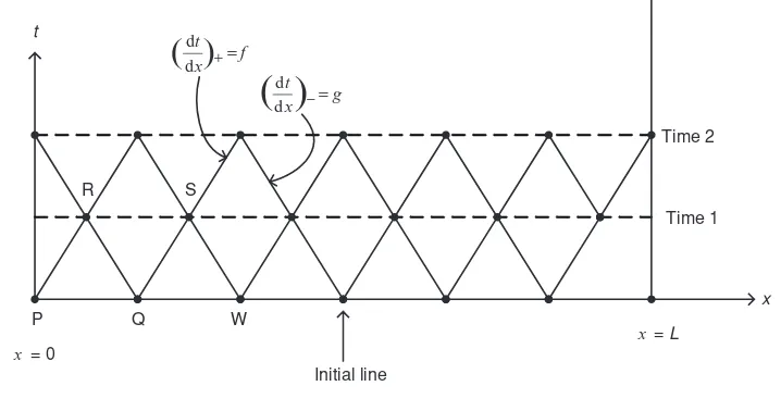
5.3.1 Numerical integration along the characteristic lines 50
5.4 Applications to financial engineering 53
5.4.1 Generalisations 55
5.5 Systems of equations 55
5.5.1 An example 57
5.6 Propagation of discontinuities 57
5.6.1 Other problems 58
Contents vii
PART II FINITE DIFFERENCE METHODS: THE FUNDAMENTALS 61
6 An Introduction to the Finite Difference Method 63
6.1 Introduction and objectives 63
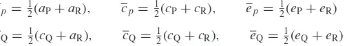
6.2 Fundamentals of numerical differentiation 63
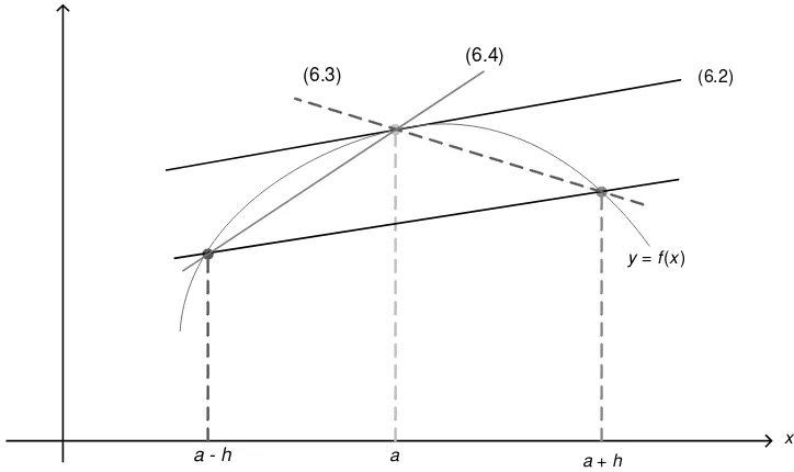
6.3 Caveat: accuracy and round-off errors 65
6.4 Where are divided differences used in instrument pricing? 67
6.5 Initial value problems 67
6.5.1 Pad´e matrix approximations 68
6.5.2 Extrapolation 71
6.6 Nonlinear initial value problems 72
6.6.1 Predictor–corrector methods 73
6.6.2 Runge–Kutta methods 74
6.7 Scalar initial value problems 75
6.7.1 Exponentially fitted schemes 76
6.8 Summary and conclusions 76
7 An Introduction to the Method of Lines 79
7.1 Introduction and objectives 79
7.2 Classifying semi-discretisation methods 79
7.3 Semi-discretisation in space using FDM 80
7.3.1 A test case 80
7.3.2 Toeplitz matrices 82
7.3.3 Semi-discretisation for convection-diffusion problems 82
7.3.4 Essentially positive matrices 84
7.4 Numerical approximation of first-order systems 85
7.4.1 Fully discrete schemes 86
7.4.2 Semi-linear problems 87
7.5 Summary and conclusions 89
8 General Theory of the Finite Difference Method 91
8.1 Introduction and objectives 91
8.2 Some fundamental concepts 91
8.2.1 Consistency 93
8.2.2 Stability 93
8.2.3 Convergence 94
8.3 Stability and the Fourier transform 94
8.4 The discrete Fourier transform 96
8.4.1 Some other examples 98
8.5 Stability for initial boundary value problems 99
8.5.1 Gerschgorin’s circle theorem 100
8.6 Summary and conclusions 101
9 Finite Difference Schemes for First-Order Partial Differential Equations 103
9.1 Introduction and objectives 103
9.3 Why first-order equations are different: Essential difficulties 105
9.3.1 Discontinuous initial conditions 106
9.4 A simple explicit scheme 106
9.5 Some common schemes for initial value problems 108
9.5.1 Some other schemes 110
9.6 Some common schemes for initial boundary value problems 110
9.7 Monotone and positive-type schemes 110
9.8 Extensions, generalisations and other applications 111
9.8.1 General linear problems 112
9.8.2 Systems of equations 112
9.8.3 Nonlinear problems 114
9.8.4 Several independent variables 114
9.9 Summary and conclusions 115
10 FDM for the One-Dimensional Convection–Diffusion Equation 117
10.1 Introduction and objectives 117
10.2 Approximation of derivatives on the boundaries 118
10.3 Time-dependent convection–diffusion equations 120
10.4 Fully discrete schemes 120
10.5 Specifying initial and boundary conditions 121
10.6 Semi-discretisation in space 121
10.7 Semi-discretisation in time 122
10.8 Summary and conclusions 122
11 Exponentially Fitted Finite Difference Schemes 123
11.1 Introduction and objectives 123
11.2 Motivating exponential fitting 123
11.2.1 ‘Continuous’ exponential approximation 124
11.2.2 ‘Discrete’ exponential approximation 125
11.2.3 Where is exponential fitting being used? 128
11.3 Exponential fitting and time-dependent convection-diffusion 128
11.4 Stability and convergence analysis 129
11.5 Approximating the derivative of the solution 131
11.6 Special limiting cases 132
11.7 Summary and conclusions 132
PART III APPLYING FDM TO ONE-FACTOR INSTRUMENT PRICING 135
12 Exact Solutions and Explicit Finite Difference Method
for One-Factor Models 137
12.1 Introduction and objectives 137
12.2 Exact solutions and benchmark cases 137
12.3 Perturbation analysis and risk engines 139
12.4 The trinomial method: Preview 139
12.4.1 Stability of the trinomial method 141
12.5 Using exponential fitting with explicit time marching 142
Contents ix
12.7 Summary and conclusions 144
12.8 Appendix: the formula for Vega 144
13 An Introduction to the Trinomial Method 147
13.1 Introduction and objectives 147
13.2 Motivating the trinomial method 147
13.3 Trinomial method: Comparisons with other methods 149
13.3.1 A general formulation 150
13.4 The trinomial method for barrier options 151
13.5 Summary and conclusions 152
14 Exponentially Fitted Difference Schemes for Barrier Options 153
14.1 Introduction and objectives 153
14.2 What are barrier options? 153
14.3 Initial boundary value problems for barrier options 154
14.4 Using exponential fitting for barrier options 154
14.4.1 Double barrier call options 156
14.4.2 Single barrier call options 156
14.5 Time-dependent volatility 156
14.6 Some other kinds of exotic options 157
14.6.1 Plain vanilla power call options 158
14.6.2 Capped power call options 158
14.7 Comparisons with exact solutions 159
14.8 Other schemes and approximations 162
14.9 Extensions to the model 162
14.10 Summary and conclusions 163
15 Advanced Issues in Barrier and Lookback Option Modelling 165
15.1 Introduction and objectives 165
15.2 Kinds of boundaries and boundary conditions 165
15.3 Discrete and continuous monitoring 168
15.3.1 What is discrete monitoring? 168
15.3.2 Finite difference schemes and jumps in time 169
15.3.3 Lookback options and jumps 170
15.4 Continuity corrections for discrete barrier options 171
15.5 Complex barrier options 171
15.6 Summary and conclusions 173
16 The Meshless (Meshfree) Method in Financial Engineering 175
16.1 Introduction and objectives 175
16.2 Motivating the meshless method 175
16.3 An introduction to radial basis functions 177
16.4 Semi-discretisations and convection–diffusion equations 177 16.5 Applications of the one-factor Black–Scholes equation 179
16.6 Advantages and disadvantages of meshless 180
17 Extending the Black–Scholes Model: Jump Processes 183
17.1 Introduction and objectives 183
17.2 Jump–diffusion processes 183
17.2.1 Convolution transformations 185
17.3 Partial integro-differential equations and financial applications 186
17.4 Numerical solution of PIDE: Preliminaries 187
17.5 Techniques for the numerical solution of PIDEs 188
17.6 Implicit and explicit methods 188
17.7 Implicit–explicit Runge–Kutta methods 189
17.8 Using operator splitting 189
17.9 Splitting and predictor–corrector methods 190
17.10 Summary and conclusions 191
PART IV FDM FOR MULTIDIMENSIONAL PROBLEMS 193
18 Finite Difference Schemes for Multidimensional Problems 195
18.1 Introduction and objectives 195
18.2 Elliptic equations 195
18.2.1 A self-adjoint elliptic operator 198
18.2.2 Solving the matrix systems 199
18.2.3 Exact solutions to elliptic problems 200
18.3 Diffusion and heat equations 202
18.3.1 Exact solutions to the heat equation 204
18.4 Advection equation in two dimensions 205
18.4.1 Initial boundary value problems 207
18.5 Convection–diffusion equation 207
18.6 Summary and conclusions 208
19 An Introduction to Alternating Direction Implicit and Splitting Methods 209
19.1 Introduction and objectives 209
19.2 What is ADI, really? 210
19.3 Improvements on the basic ADI scheme 212
19.3.1 The D’Yakonov scheme 212
19.3.2 Approximate factorization of operators 213
19.3.3 ADI classico for two-factor models 215
19.4 ADI for first-order hyperbolic equations 215
19.5 ADI classico and three-dimensional problems 217
19.6 The Hopscotch method 218
19.7 Boundary conditions 219
19.8 Summary and conclusions 221
20 Advanced Operator Splitting Methods: Fractional Steps 223
20.1 Introduction and objectives 223
20.2 Initial examples 223
20.3 Problems with mixed derivatives 224
20.4 Predictor–corrector methods (approximation correctors) 226
Contents xi
20.6 More general results 228
20.7 Summary and conclusions 228
21 Modern Splitting Methods 229
21.1 Introduction and objectives 229
21.2 Systems of equations 229
21.2.1 ADI and splitting for parabolic systems 230
21.2.2 Compound and chooser options 231
21.2.3 Leveraged knock-in options 232
21.3 A different kind of splitting: The IMEX schemes 232
21.4 Applicability of IMEX schemes to Asian option pricing 234
21.5 Summary and conclusions 235
PART V APPLYING FDM TO MULTI-FACTOR INSTRUMENT PRICING 237
22 Options with Stochastic Volatility: The Heston Model 239
22.1 Introduction and objectives 239
22.2 An introduction to Ornstein–Uhlenbeck processes 239
22.3 Stochastic differential equations and the Heston model 240
22.4 Boundary conditions 241
22.4.1 Standard european call option 242
22.4.2 European put options 242
22.4.3 Other kinds of boundary conditions 242
22.5 Using finite difference schemes: Prologue 243
22.6 A detailed example 243
22.7 Summary and conclusions 246
23 Finite Difference Methods for Asian Options and Other ‘Mixed’ Problems 249
23.1 Introduction and objectives 249
23.2 An introduction to Asian options 249
23.3 My first PDE formulation 250
23.4 Using operator splitting methods 251
23.4.1 For sake of completeness: ADI methods for asian option PDEs 253
23.5 Cheyette interest models 253
23.6 New developments 254
23.7 Summary and conclusions 255
24 Multi-Asset Options 257
24.1 Introduction and objectives 257
24.2 A taxonomy of multi-asset options 257
24.2.1 Exchange options 260
24.2.2 Rainbow options 261
24.2.3 Basket options 262
24.2.4 The best and worst 263
24.2.5 Quotient options 263
24.2.6 Foreign equity options 264
24.2.8 Spread options 264
24.2.9 Dual-strike options 265
24.2.10 Out-perfomance options 265
24.3 Common framework for multi-asset options 265
24.4 An overview of finite difference schemes for multi-asset problems 266
24.5 Numerical solution of elliptic equations 267
24.6 Solving multi-asset Black–Scholes equations 269
24.7 Special guidelines and caveats 270
24.8 Summary and conclusions 271
25 Finite Difference Methods for Fixed-Income Problems 273
25.1 Introduction and objectives 273
25.2 An introduction to interest rate modelling 273
25.3 Single-factor models 274
25.4 Some specific stochastic models 276
25.4.1 The Merton model 277
25.4.2 The Vasicek model 277
25.4.3 Cox, Ingersoll and Ross (CIR) 277
25.4.4 The Hull–White model 277
25.4.5 Lognormal models 278
25.5 An introduction to multidimensional models 278
25.6 The thorny issue of boundary conditions 280
25.6.1 One-factor models 280
25.6.2 Multi-factor models 281
25.7 Introduction to approximate methods for interest rate models 282
25.7.1 One-factor models 282
25.7.2 Many-factor models 283
25.8 Summary and conclusions 283
PART VI FREE AND MOVING BOUNDARY VALUE PROBLEMS 285
26 Background to Free and Moving Boundary Value Problems 287
26.1 Introduction and objectives 287
26.2 Notation and definitions 287
26.3 Some preliminary examples 288
26.3.1 Single-phase melting ice 288
26.3.2 One-factor option modelling: American exercise style 289
26.3.3 Two-phase melting ice 290
26.3.4 The inverse Stefan problem 290
26.3.5 Two and three space dimensions 291
26.3.6 Oxygen diffusion 293
26.4 Solutions in financial engineering: A preview 293
26.4.1 What kinds of early exercise features? 293
26.4.2 What kinds of numerical techniques? 294
Contents xiii
27 Numerical Methods for Free Boundary Value Problems:
Front-Fixing Methods 295
27.1 Introduction and objectives 295
27.2 An introduction to front-fixing methods 295
27.3 A crash course on partial derivatives 295
27.4 Functions and implicit forms 297
27.5 Front fixing for the heat equation 299
27.6 Front fixing for general problems 300
27.7 Multidimensional problems 300
27.8 Front fixing and American options 303
27.9 Other finite difference schemes 305
27.9.1 The method of lines and predictor–corrector 305
27.10 Summary and conclusions 306
28 Viscosity Solutions and Penalty Methods for American Option Problems 307
28.1 Introduction and objectives 307
28.2 Definitions and main results for parabolic problems 307
28.2.1 Semi-continuity 307
28.2.2 Viscosity solutions of nonlinear parabolic problems 308 28.3 An introduction to semi-linear equations and penalty method 310
28.4 Implicit, explicit and semi-implicit schemes 311
28.5 Multi-asset American options 312
28.6 Summary and conclusions 314
29 Variational Formulation of American Option Problems 315
29.1 Introduction and objectives 315
29.2 A short history of variational inequalities 316
29.3 A first parabolic variational inequality 316
29.4 Functional analysis background 318
29.5 Kinds of variational inequalities 319
29.5.1 Diffusion with semi-permeable membrane 319
29.5.2 A one-dimensional finite element approximation 320
29.6 Variational inequalities using Rothe’s methods 323
29.7 American options and variational inequalities 324
29.8 Summary and conclusions 324
PART VII DESIGN AND IMPLEMENTATION IN C++ 325
30 Finding the Appropriate Finite Difference Schemes for your Financial
Engineering Problem 327
30.1 Introduction and objectives 327
30.2 The financial model 328
30.3 The viewpoints in the continuous model 328
30.3.1 Payoff functions 329
30.3.2 Boundary conditions 330
30.4 The viewpoints in the discrete model 332
30.4.1 Functional and non-functional requirements 332
30.4.2 Approximating the spatial derivatives in the PDE 333
30.4.3 Time discretisation in the PDE 334
30.4.4 Payoff functions 334
30.4.5 Boundary conditions 335
30.5 Auxiliary numerical methods 335
30.6 New Developments 336
30.7 Summary and conclusions 336
31 Design and Implementation of First-Order Problems 337
31.1 Introduction and objectives 337
31.2 Software requirements 337
31.3 Modular decomposition 338
31.4 Useful C++data structures 339
31.5 One-factor models 339
31.5.1 Main program and output 342
31.6 Multi-factor models 343
31.7 Generalisations and applications to quantitative finance 346
31.8 Summary and conclusions 347
31.9 Appendix: Useful data structures in C++ 348
32 Moving to Black–Scholes 353
32.1 Introduction and objectives 353
32.2 The PDE model 354
32.3 The FDM model 355
32.4 Algorithms and data structures 355
32.5 The C++model 356
32.6 Test case: The two-dimensional heat equation 357
32.7 Finite difference solution 357
32.8 Moving to software and method implementation 358
32.8.1 Defining the continuous problem 358
32.8.2 Creating a mesh 358
32.8.3 Choosing a scheme 360
32.8.4 Termination criterion 361
32.9 Generalisations 361
32.9.1 More general PDEs 361
32.9.2 Other finite difference schemes 361
32.9.3 Flexible software solutions 361
32.10 Summary and conclusions 362
33 C++Class Hierarchies for One-Factor and Two-Factor Payoffs 363
33.1 Introduction and objectives 363
33.2 Abstract and concrete payoff classes 364
33.3 Using payoff classes 367
33.4 Lightweight payoff classes 368
Contents xv
33.6 Payoff functions for multi-asset option problems 371
33.7 Caveat: non-smooth payoff and convergence degradation 373
33.8 Summary and conclusions 374
Appendices 375
A1 An introduction to integral and partial integro-differential equations 375 A2 An introduction to the finite element method 393
Bibliography 409
0
Goals of this Book and Global Overview
0.1 WHAT IS THIS BOOK?
The goal of this book is to develop robust, accurate and efficient numerical methods to price a number of derivative products in quantitative finance. We focus on one-factor and multi-factor models for a wide range of derivative products such as options, fixed income products, interest rate products and ‘real’ options. Due to the complexity of these products it is very difficult to find exact or closed solutions for the pricing functions. Even if a closed solution can be found it may be very difficult to compute. For this and other reasons we need to resort to approximate methods. Our interest in this book lies in the application of the finite difference method (FDM) to these problems.
This book is a thorough introduction to FDM and how to use it to approximate the various kinds of partial differential equations for contingent claims such as:
r
One-factor European and American optionsr
One-factor and two-factor barrier options with continuous and discrete monitoringr
Multi-asset optionsr
Asian options, continuous and discrete monitoringr
One-factor and two-factor bond optionsr
Interest rate modelsr
The Heston model and stochastic volatilityr
Merton jump models and extensions to the Black–Scholes model.Finite difference theory has a long history and has been applied for more than 200 years to approximate the solutions of partial differential equations in the physical sciences and engineering.
What is the relationship between FDM and financial engineering? To answer this ques-tion we note that the behaviour of a stock (or some other underlying) can be described by a stochastic differential equation. Then, a contingent claim that depends on the underlying is modelled by a partial differential equation in combination with some initial and bound-ary conditions. Solving this problem means that we have found the value for the contingent claim.
Furthermore, we discuss finite difference and variational schemes that model free and mov-ing boundaries. This is the style for exercismov-ing American options, and we employ a number of new modelling techniques to locate the position of the free boundary.
Finally, we introduce and elaborate the theory of partial integro-differential equations (PIDEs), their applications to financial engineering and their approximations by FDM. In particular, we show how the basic Black–Scholes partial differential equation is augmented by an integral term in order to model jumps (the Merton model). Finally, we provide worked-out
0.2 WHY HAS THIS BOOK BEEN WRITTEN?
There are a number of reasons why this book has been written. First, the author wanted to produce a text that showed how to apply numerical methods (in this case, finite difference schemes) to quantitative finance. Furthermore, it is important to justify the applicability of the schemes rather than just rely on numerical recipes that are sometimes difficult to apply to real problems. The second desire was to construct robust finite difference schemes for use in financial engineering, creating algorithms that describe how to solve the discrete set of
equations that result from such schemes and then to map them to C++code.
0.3 FOR WHOM IS THIS BOOK INTENDED?
This book is for quantitative analysts, financial engineers and others who are involved in defining and implementing models for various kinds of derivatives products. No previous knowledge of partial differential equations (PDEs) or of finite difference theory is assumed. It is, however, assumed that you have some knowledge of financial engineering basics, such as stochastic differential equations, Ito calculus, the Black–Scholes equation and derivative pricing in general. This book will be of value to those financial engineers who use the binomial and trinomial methods to price options, as these two methods are special cases of explicit finite difference schemes. This book will also hopefully be employed by those engineers who use simulation methods (for example, the Monte Carlo method) to price derivatives, and it is hoped that the book will help to bridge the gap between the stochastics and PDE approaches.
Finally, this book could be interesting for mathematicians, physicists and engineers who wish to see how a well-known branch of numerical analysis is applied to financial engineering. The information in the book may even improve your job prospects!
0.4 WHY SHOULD I READ THIS BOOK?
In the author’s opinion, this is one of the first self-contained introductions to the finite difference method and its applications to derivatives pricing. The book introduces the theory of PDE and FDM and their applications to quantitative finance, and can be used as a self-contained guide to learning and discovering the most important finite difference schemes for derivative pricing problems.
Some of the advantages of the approach and the resulting added value of the book are:
r
A defined process starting from the financial models through PDEs, FDM and algorithmsr
An application of robust, accurate and efficient finite difference schemes for derivativespricing applications.
This book is more than just a cookbook: it motivates why a method does or does not work and you can learn from this knowledge in a meaningful way. This book is also a good companion
to my other book,Financial Instrument Pricing in C++(Duffy, 2004). The algorithms in
the present book can be mapped to C++, the de-facto object-oriented language for financial engineering applications
Goals of this Book and Global Overview 3
0.5 THE STRUCTURE OF THIS BOOK
The book has been partitioned into seven parts, each of which deals with one specific topic in detail. Furthermore, each part contains material that is required by its successor. In general, we interleave the parts by first discussing the theory (for example, basic finite difference schemes) in a given part and then applying this theory to a problem in financial engineering. This ‘separation of concerns’ approach promotes understandability of the material, and the parts in the book discuss the following topics:
I. The Continuous Theory of Partial Differential Equations
II. Finite Difference Methods: the Fundamentals
III. Applying FDM to One-Factor Instrument Pricing
IV. FDM for Multidimensional Problems
V. Applying FDM to Multi-Factor Instrument Pricing
VI. Free and Moving Boundary Value Problems
VII. Design and Implementation in C++
Part Ipresents an introduction to partial differential equations (PDE). This theory may be new for some readers and for this reason these equations are discussed in some detail. The relevance of PDE to instrument pricing is that a contingent claim or derivative can be modelled as an initial boundary value problem for a second-order parabolic partial differential equation. The partial differential equation has one time variable and one or more space variables. The focus in Part I is to develop enough mathematical theory to provide a basis for work on finite differences.
Part IIis an introduction to the finite difference method for a number of partial differential equations that appear in instrument pricing problems. We learn FDM in the following way: (1) We introduce the model PDEs for the heat, convection and convection–diffusion equations and propose several important finite difference schemes to approximate them. In particular, we discuss a number of schemes that are used in the financial engineering literature and we also introduce some special schemes that work under a range of parameter values. In this part, focus is on the practical application of FDM to parabolic partial differential equations in one space variable.
Part III examines the partial differential equations that describe one-factor instrument models and their approximation by the finite difference schemes. In particular, we concen-trate on European options, barrier options and options with jumps, and propose several finite difference schemes for such options. An important class of problems discussed in this part is the class of barrier options with continuous or discrete monitoring and robust methods are proposed for each case. Finally, we model the partial integro-differential equations (PIDEs) that describe options with jumps, and we show how to approximate them by finite difference schemes.
Part Vapplies the results and schemes from Part IV to approximating some multi-factor problems. In particular, we examine the Heston PDE with stochastic volatility, Asian options, rainbow options and two-factor bond models and how to apply ADI and operator splitting methods to them.
Part VIdeals with instrument pricing problems with the so-called early exercise feature. Mathematically, these problems fall under the umbrella of free and moving boundary value problems. We concentrate on the theory of such problems and the application to one-factor American options. We also discuss ADI method in conjunction with free boundaries.
Part VIIcontains a number of chapters that support the work in the previous parts of the book. Here we address issues that are relevant to the design and implementation of the FDM algorithms in the book. We provide hints, guidelines and C++sources to help the reader to make the transition to production code.
0.6 WHAT THIS BOOK DOES NOT COVER
This book is concerned with the application of the finite difference method to instrument pricing. This viewpoint implies that we concentrate on a number of issues while neglecting others. Thus, this book is not:
r
an introduction to numerical analysisr
a guide to the theoretical foundations of the theory of finite differencesr
an introduction to instrument pricingr
a full ‘production’ C++course.These problems are considered in detail in other books and will be discussed elsewhere.
0.7 CONTACT, FEEDBACK AND MORE INFORMATION
The author welcomes your feedback, comments and suggestions for improvement. As far as I am aware, all typos and errors have been removed from the text, but some may have slipped past unnoticed. Nevertheless, all errors are my responsibility.I am a trainer and developer and my main professional interests are in quantitative finance, computational finance and object-oriented programming. In my free time I enjoy judo and studying foreign (natural) languages.
Part I
1
An Introduction to Ordinary
Differential Equations
1.1 INTRODUCTION AND OBJECTIVES
Part I of this book is devoted to an overview of ordinary and partial differential equations. We discuss the mathematical theory of these equations and their relevance to quantitative finance. After having read the chapters in Part I you will have gained an appreciation of one-factor and multi-factor partial differential equations.
In this chapter we introduce a class ofsecond-order ordinary differential equationsas they contain derivatives up to order 2 in one independent variable. Furthermore, the (unknown) function appearing in the differential equation is a function of a single variable. A simple example is thelinearequation
Lu≡a(x)u′′+b(x)u′+c(x)u= f(x) (1.1)
In general we seek a solutionuof (1.1) in conjunction with some auxiliary conditions. The coefficientsa,b,cand f are known functions of the variablex. Equation (1.1) is called linear because all coefficients are independent of the unknown variableu. Furthermore, we have used the following shorthand for the first- and second-order derivatives with respect tox:
u′= du
dx and u ′′
= d
2u
dx2 (1.2)
We examine (1.1) in some detail in this chapter because it is part of the Black–Scholes equation
∂C ∂t +
1 2σ
2S2∂2C
∂S2 +r S
∂C
∂S −r C =0 (1.3)
where the asset price S plays the role of the independent variablex andt plays the role of time. We replace the unknown functionubyC (the option price). Furthermore, in this case, the coefficients in (1.1) have the special form
a(S) = 12σ2S2
b(S) =r S c(S) = −r f(S)=0
(1.4)
1.2 TWO-POINT BOUNDARY VALUE PROBLEM
Let us examine a general second-order ordinary differential equation given in the form
u′′= f(x;u,u′) (1.5)
where the function f depends on three variables. The reader may like to check that (1.1) is a special case of (1.5). In general, there will be many solutions of (1.5) but our interest is in defining extra conditions to ensure that it will have a unique solution. Intuitively, we might correctly expect that two conditions are sufficient, considering the fact that you could integrate (1.5) twice and this will deliver two constants of integration. To this end, we determine these extra conditions by examining (1.5) on aboundedinterval (a,b). In general, we discuss linear combinations of the unknown solutionuand its first derivative at these end-points:
a0u(a)−a1u′(a)=α , |a0| + |a1| =0
b0u(b)+b1u′(b)=β , |b0| + |b1| =0
(1.6)
We wish to know the conditions under which problem (1.5), (1.6) has a unique solution. The full treatment is given in Keller (1992), but we discuss the main results in this section. First, we need to place some restrictions on the function f that appears on the right-hand side of equation (1.5).
Definition 1.1. The function f(x,u, v) is called uniformly Lipschitz continuous if
|f(x;u,v)− f(x;w,z)| ≤Kmax(|u−w|,|v−z|) (1.7) whereK is some constant, andx,ut, andvare real numbers.
We now state the main result (taken from Keller, 1992).
Theorem 1.1. Consider the function f(x;u, v) in (1.5) and suppose that it is uniformly Lipschitz continuous in the region R, defined by:
R:a≤x≤b, u2+v2<∞ (1.8)
Suppose, furthermore, that f has continuous derivatives in R satisfying, for some constant M,
∂f ∂u >0,
∂f ∂v
≤M (1.9)
and, that
a0a1 ≥0, b0b1≥0, |a0| + |b0| =0 (1.10)
Then the boundary-value problem(1.5), (1.6)has a unique solution.
This is a general result and we can use it in new problems to assure us that they have a unique solution.
1.2.1 Special kinds of boundary condition
An Introduction to Ordinary Differential Equations 9
the Black–Scholes equation. The main categories are:
r
Robin boundary conditionsr
Dirichlet boundary conditionsr
Neumann boundary conditions.The most general of those is the Robin condition, which is, in fact, (1.6). Special cases of (1.6) at the boundariesx=aorx=bare formed by setting some of the coefficients to zero. For example, the boundary conditions at the end-pointx=a:
u(a)=α
u′(a)=β (1.11)
are called Dirichlet and Neumann boundary conditions atx=aand atx=b, respectively. Thus, in the first case the value of the unknown functionuis known atx=awhile, in the second case, its derivative is known atx=b(but notuitself). We shall encounter the above three types of boundary condition in this book, not only in a one-dimensional setting but also in multiple dimensions. Furthermore, we shall discuss other kinds of boundary condition that are needed in financial engineering applications.
1.3 LINEAR BOUNDARY VALUE PROBLEMS
We now consider a special case of (1.5), namely (1.1). This is called alinear equationand is important in many kinds of applications. A special case of Theorem 1.1 occurs when the function f(x;u, v) is linear in bothuandv. For convenience, we write (1.1) in the canonical form
−u′′+p(x)u′+q(x)u= r(x) (1.12)
and the result is:
Theorem 1.2. Let the functions p(x),q(x)and r(x)be continuous in the closed interval[a,b] with
q(x)>0, a ≤x≤b, a0a1≥0, |a0| + |a1| =0,
b0b1≥0, |b0| + |b1| =0,
(1.13)
Assume that
|a0| + |b0| =0
then the two-point boundary value problem (BVP)
Lu≡ −u′′+p(x)u′+q(x)u=r(x), a<x<b a0u(a)−a1u′(a)=α, b0u(b)+b1u′(b)=β
(1.14)
has a unique solution.
Remark. The condition |a0| + |b0| =0 excludes boundary value problems with Neumann
1.4 INITIAL VALUE PROBLEMS
In the previous section we examined a differential equation on a bounded interval. In this case we assumed that the solution was defined in this interval and that certain boundary conditions were defined at the interval’s end-points. We now consider a different problem where we wish to find the solution on a semi-infinite interval, let’s say (a,∞). In this case we define the initial value problem (IVP)
u′′= f(x;u,u′)
a0u(a)−a1u′(a)=α
b0u(a)−b1u′(a)=β
(1.15)
where we assume that the two conditions atx=aare independent, that is
a1b0−a0b1=0 (1.16)
It is possible to write (1.15) as a first-order system by a change of variables:
u′=v, v′= f(x;u, v)
a0u(a)−a1v(a)=α
b0u(a)−b1v(a)=β
(1.17)
This is now a first-order system containing no explicit derivatives atx=a. System (1.17) is in a form that can be solved numerically by standard schemes (Keller, 1992). In fact, we can apply the same transformation technique to the boundary value problem (1.14) to get
−v′+p(x)v+q(x)u =r(x)
u′=v
a0u(a)−a1v(a)=α,
b0u(b)+b1v(b)=β
(1.18)
This approach has a number of advantages when we apply finite difference schemes to approximate the solution of problem (1.18). First, we do not need to worry about approximating derivatives at the boundaries and, second, we are able to approximatevwith the same accuracy asu itself. This is important in financial engineering applications because the first derivative represents an option’s delta function.
1.5 SOME SPECIAL CASES
There are a number of common specialisations of equation (1.5), and each has its own special name, depending on its form:
Reaction–diffusion: u′′=q(x)u
Convection–diffusion: u′′=p(x)u′
Diffusion: u′′=0
(1.19)
An Introduction to Ordinary Differential Equations 11
has applications to fluid dynamics, semiconductor modelling and groundwater flow, to name just a few (Morton, 1996). It is also an essential part of the Black–Scholes equation (1.3).
We can transform equation (1.1) into a more convenient form (the so-callednormal form) by a change of variables under the constraint that the coefficient of the second derivativea(x) is always positive. For convenience we assume that the right-hand side term f is zero. To this end, define
p(x)=exp b(x)
a(x)dx
(1.20) q(x)= c(x)p(x)
a(x)
If we multiply equation (1.1) (note f =0) byp(x)/a(x) we then get: d
dxp(x) du
dx +q(x)u=0 (1.21)
This is sometimes known as theself-adjoint form. A further change of variables
ζ =
dx
p(x) (1.22)
allows us to write (1.21) to an even simpler form d2u
dζ2 +p(x)q(x)u =0 (1.23)
Equation (1.23) is simpler to solve than equation (1.1).
1.6 SUMMARY AND CONCLUSIONS
2
An Introduction to Partial
Differential Equations
2.1 INTRODUCTION AND OBJECTIVES
In this chapter we give a gentle introduction to partial differential equations (PDEs). It can be considered to be a panoramic view and is meant to introduce some notation and examples. A PDE is an equation that depends on several independent variables. A well-known example is the Laplace equation:
∂2u ∂x2 +
∂2u
∂y2 =0 (2.1)
In this case the dependent variableusatisfies (2.1) in some bounded, infinite or semi-infinite space in two dimensions.
In this book we examine PDEs in one or more space dimensions and a single time dimension. An example of a PDE with a derivative in the time direction is the heat equation in two spatial dimensions:
∂u ∂t =
∂2u ∂x2 +
∂2u
∂y2 (2.2)
We classify PDEs into three categories of equation, namely parabolic, hyperbolic and elliptic. Parabolic equations are important for financial engineering applications because the Black–Scholes equation is a specific instance of such a category. Furthermore, generalisations and extensions to the Black–Scholes model may have hyperbolic equations as components. Finally, elliptic equations are useful because they form the time-independent part of the Black– Scholes equations.
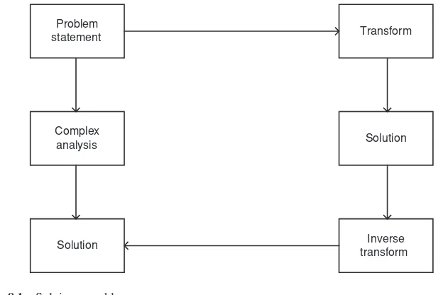
2.2 PARTIAL DIFFERENTIAL EQUATIONS
We have attempted to categorise partial differential equations as shown in Figure 2.1. At the highest level we have the three major categories already mentioned. At the second level we have classes of equation based on the orders of the derivatives appearing in the PDE, while at level three we have given examples that serve as model problems for more complex equations. The hierarchy is incomplete and somewhat arbitrary (as all taxonomies are). It is not our intention to discuss all PDEs that are in existence but rather to give the reader an overview of some different types. This may be useful for readers who may not have had exposure to such equations in the past.
What makes a PDE parabolic, hyperbolic or elliptic? To answer this question let us examine thelinearpartial differential equation in two independent variables (Carrier and Pearson, 1976; Petrovsky, 1991)
PDE
Parabolic Elliptic Hyperbolic
Convection–diffusion
Black–Scholes
Diffusion
Heat equation
Poisson
Laplace
1st order
Shocks Hamilton–Jacobi Friedrichs’ systems
2nd order
Wave equation
Figure 2.1 PDE classification
where we have used the (common) shorthand notation
ux =
∂u
∂x, uy= ∂u ∂y ux x=
∂2u
∂x2, uyy=
∂2u ∂y2
ux y =
∂2u ∂x∂y
(2.4)
and the coefficientsA,B,C,D,E,FandGare functions ofxandyin general. Equation (2.3) is linear because these functions do not have a dependency on the unknown function u=
u(x,y). We assume that equation (2.3) is specified in some region of (x,y) space. Note the presence of the cross (mixed) derivatives in (2.3). We shall encounter these terms again in later chapters.
Equation (2.3) subsumes well-known equations in mathematical physics as special cases. For example, the Laplace equation (2.1) is a special case, having the following values:
A=C =1
B=D=E =F=G=0 (2.5)
A detailed discussion of (2.3), and the conditions that determine whether it is elliptic, hyperbolic or parabolic, is given in Carrier and Pearson (1976). We give the main results in this section. The discussion in Carrier and Pearson (1976) examines the quadratic equation:
Aξx2+2Bξxξy+Cξy2=0 (2.6)
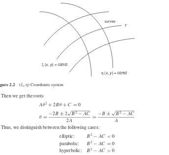
whereξ(x,y) is some family of curves in (x,y) space (see Figure 2.2). In particular, we wish to find the solutions of the quadratic form by defining the variables:
θ =ξx
ξy
An Introduction to Partial Differential Equations 15
curves
ξ (x, y) = const
η (x, y) = const
Γ
Figure 2.2 (ξ,η) Coordinate system
Then we get the roots
Aθ2+2Bθ+C=0
θ= −2B±2
√
B2−AC
2A =
−B±√B2−AC
A
(2.8)
Thus, we distinguish between the following cases: elliptic: B2−AC<0 parabolic: B2
−AC=0 hyperbolic: B2−AC>0
(2.9)
We note that the variablesxandyappearing in (2.3) are generic and in some cases we may wish to replace them by other more specific variables – for example, replacing yby a time variabletas in the well-known one-dimensional wave equation
∂2u ∂t2 −
∂2u
∂x2 =0 (2.10)
It is easy to check that in this case the coefficients are: A=1, C= −1, B=D=E = F=G=0 and hence the equation is hyperbolic.
2.3 SPECIALISATIONS
We now discuss a number of special cases of elliptic, parabolic and hyperbolic equations that occur in many areas of application. These equations have been discovered and investigated by the greatest mathematicians of the last three centuries and there is an enormous literature on the theory of these equations and their applications to the world around us.
2.3.1 Elliptic equations
These time-independent equations occur in many kinds of application:
r
Steady-state heat conduction (Kreideret al., 1966)Γ
ηΩ
Figure 2.3 Two-dimensional bounded region
r
Harmonic functions (Du Plessis, 1970; Rudin, 1970)r
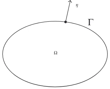
Mapping functions between two-dimensional regions (George, 1991).In general, we must specify boundary conditions for elliptic equations if we wish to have a unique solution. To this end, let us consider a two-dimensional regionwith smooth boundary Ŵas shown in Figure 2.3, and letηbe the positive outward normal vector onŴ. A famous example of an elliptic equation is the Poisson equation defined by:
u≡ ∂
2u
∂x2 +
∂2u
∂y2 = f(x,y) in (2.11)
whereis the Laplace operator.
Equation (2.11) has a unique solution if we define boundary conditions. There are various options, the most general of which is the Robin condition:
α∂u
∂η+βu=g (2.12)
whereα, βandgare given functions defined on the boundaryŴ. A special case is whenα=0, in which case (2.12) reduces to Dirichlet boundary conditions.
A special case of the Poisson equation (2.11) is when f =0. This is then called the Laplace equation (2.1).
In general, we must resort to numerical methods if we wish to find a solution of prob-lem (2.11), (2.12). For general domains, the finite eprob-lement method (FEM) and other so-called variational techniques have been applied with success (see, for example, Stranget al., 1973; Hughes, 2000). In this book we are mainly interested in square and rectangular regions be-cause many financial engineering applications are defined in such regions. In this case the finite difference method (FDM) is our method of choice (see Richtmyer and Morton, 1967).
An Introduction to Partial Differential Equations 17
2.3.2 Free boundary value problems
In the previous section we assumed that the boundaryŴof the domain of interest is known. In many applications, however, we not only need to find the solution of a PDE in some region but we define auxiliary constraints on someunknownboundary. This boundary may be internal or external to the domain. For time-independent problems we speak of free boundaries while for time-dependent problems we use the term ‘moving’ boundaries. These boundaries occur in numerous applications, some of which are:
r
Flow in dams (Baiocchi, 1972; Friedman, 1979)r
Stefan problem: standard model for the melting of ice (Crank, 1984)r
Flow in porous media (Huyakorn and Pinder, 1983)r
Early exercise and American style option (Nielsonet al., 2002).The following is a good example of a free boundary problem. Imagine immersing a block of ice in luke-warm water at timet=0. Of course, the ice block eventually disappears because of its state change to water. The interesting question is: What is the profile of the block at any time aftert =0? This is a typical moving boundary value problem.
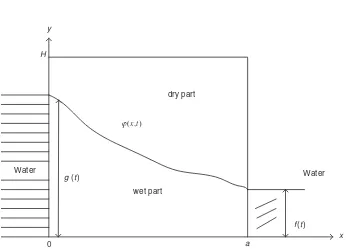
Another example that is easy to understand is the following. Consider a rectangular dam D= {(x,y) : 0<x<a, 0<y<H}and suppose that the wallsx =0 andx=aborder reservoirs of water maintained at given levelsg(t) and f(t), respectively (see Figure 2.4). The so-called piezometric head is given byu=u(x,y,t)=y+p(x,y,t), wherepis the pressure in the dam. The velocity components are given by:
velocity of water = −(ux,uy) (2.13)
y
x H
a Water
dry part
Water g (t)
wet part
f(t)
0
) , (xt ϕ
Furthermore, we distinguish between the dry part and the wet part of the dam as defined by the functionϕ(x,t). The defining equations are (Friedman, 1979; Magenes, 1972):
∂2u ∂x2 +
∂2u
∂y2 =0 if 0<x<a, 0<y< ϕ(x,t), t >0
u(0,y,t)=g(t), 0<y<g(t) u(0,y,t)=y, g(t)<y< ϕ(0, t) u(a,y,t)= f(t), 0<y< f(t) u(a,y,t)=y, f(t)<y< ϕ(a, t) uy(x,0,t)=0, 0<x<a, t>0
(2.14)
The functionϕ(x,t) is called the free boundary and it separates the wet part from the dry part of the dam.
Furthermore, on the free boundaryy=ϕ(x,t) we have the following conditions: u=y
ut =u2x+u2y−uy
(2.15)
Finally, we have the initial conditions:
ϕ(x,0)=ϕ0(x), 0≤x ≤a
ϕ0(x)>0, ϕ0(0)≥g(0), ϕ0(a)≥ f(0)
(2.16)
We thus see that the problem is the solution of the Laplace equation in the wet region of the dam while, on the free boundary, the equation is a first-order nonlinear hyperbolic equation. Thus, the free boundary is part of the problem and it must be evaluated.
A discussion of analytic and numerical methods for free and moving boundary value prob-lems is given in Crank (1984). Free and moving boundary probprob-lems are extremely important in financial engineering, as we shall see in later chapters.
A special case of (2.14) is the so-called stationary dam problem (Baiocchi, 1972). In this case the levels of the reservoirs do not change and we then have the special cases
g(t)≡g(0) f(t)≡ f(0)
andy=ϕ0(x) is the free boundary.
There may be similarities between the above problem and the free boundary problems that we encounter when modelling options with early excercise features.
2.4 PARABOLIC PARTIAL DIFFERENTIAL EQUATIONS
This is the most important PDE category in this book because of its relationship to the Black– Scholes equation. The most general linear parabolic PDE inn dimensions in this context is given by
∂u ∂t =Lu Lu≡
n
i,j=1
ai,j(x,t)
∂2u ∂xi∂xj +
n
j=1
bj(x,t)
∂u ∂xj +
cu
An Introduction to Partial Differential Equations 19
wherexis a point inn-dimensional real space andtis the time variable, wheretis increasing fromt=0. We assume that the operatorL isuniformly elliptical, that is, there exist positive constantsαandβ such that
α|ξ|2≤
forxin some region ofn-dimensional space andt ≥0. Another way of expressing (2.18) is by saying that matrixA, defined by
A=(ai,j)ni,j=1 (2.19)
is positive-definite.
A special case of (2.17) is the famous multivariate Black–Scholes equation
∂C
whereτis the time left to the expiryT andCis the value of the option onnunderlying assets. The other parameters and coefficients are:
σj =volatility of assetj
ρi j=correlation between asseti and asset j
r =risk-free intererst rate dj =dividend yield of thejth asset
(2.21)
Equation (2.20) can be derived from the following stochastic differential equation (SDE):
dSj=(μj−dj)Sjdt+σjSjdzj (2.22)
and using the generalised Ito’s lemma (see, for example, Bhansali, 1998).
In general, we need to define a unique solution to (2.17) by augmenting the equation with initial conditions and boundary conditions. We shall deal with these in later chapters but for the moment we give one example of a parabolic initial boundary value problem (IBVP) on a bounded domainwith boundaryŴ. This is defined as the PDE augmented with the following extra boundary and initial conditions
α∂u
∂η +βu =g on Ŵ×(0,T) u(x,0)=u0(x), xǫ
(2.24)
whereis the closure of.
introduce finite difference schemes for these problems; and finally we examine their relevance to financial engineering.
2.4.1 Special cases
The second-order terms in (2.17) are called diffusion termswhile the first-order terms are calledconvection(or advection) terms. If the convection terms are zero we then arrive at a diffusion equation, and if the diffusion terms are zero we then arrive at a first-order (hyperbolic) convection equation.
An even more special case of a diffusion equation is when all the diffusion coefficients are equal to 1. We then arrive at the heat equation in non-dimensional form. For example, in three space dimensions this equation has the form
∂u
A special class of equations is calledconvection–diffusion. A prototypical example in one space dimension is
Convection–diffusion equations will receive much attention in this book because they model the behaviour of one-factor option pricing problems.
2.5 HYPERBOLIC EQUATIONS
Whereas parabolic equations model fluid and heat flow phenomena, hyperbolic equations model wave phenomena, and there are many application areas where hyperbolic wave equations play an important role:
r
Shock waves (Lax, 1973)r
Acoustics (Kinsleret al., 1982)r
Neutron transport phenomena (Richtmyer and Morton, 1967)r
Deterministic models in quantitative finance (for example, deterministic interest rates). We are interested in two sub-categories, namely second-order and first-order hyperbolic equa-tions.2.5.1 Second-order equations
In this case we have a PDE containing a second-order derivative in time. A typical example is the equation (written in self-adjoint form)
∂2u
An Introduction to Partial Differential Equations 21
We now take a specific example. Consider an infinite stretched rod of negligible mass. The equations for the displacement of the string given a certain displacement are given by:
∂2u
A common procedure when viewing (2.28) both analytically and numerically is to define new variablesvandw:
v= ∂u
∂x and w= ∂u
∂t (2.29)
We can write equations (2.28) as a first-order system:
A∂U ∂t +B
∂U
∂x +CU =0 (2.30)
where we define the vectors
U =
It can be advantageous from both an analytical and numerical viewpoint to transform higher-order equations to a first-higher-order system.
2.5.2 First-order equations
First-order hyperbolic equations occur in many applications, especially in the theory of gas flow and in shock waves. The prototypical scalar initial value problem is
∂u
Furthermore, the smoothness of the solution of (2.33) is determined by its discontinuities (determined by the continuity of the initial condition) and these will be propagated indefinitely. This is different from parabolic PDEs where discontinuities in the initial condition become smeared out as time goes on.
2.6 SYSTEMS OF EQUATIONS
In some applications we may wish to solve a PDE for vector-valued functions, that is sys-tems of equations. We shall also come across some examples of such syssys-tems in the finan-cial engineering applications in this book. Typical cases are chooser options and compound options.
2.6.1 Parabolic systems
Let us consider the two-dimensional problem
∂U ∂t =A
∂2U ∂x2 +B
∂2U ∂y2 +C
∂U ∂x +D
∂U
∂y +EU (2.34)
whereUis a vector of unknowns andA,B,C,DandEare matrices. We say that the system (2.34) is parabolic if for each vectorw∈R2
w=t(w1, w2) the eigenvaluesKj(w), j =1, . . . ,nof −w12A−w22B (2.35)
satisfy ReKj(w)≤δ|w|2, j=1, . . . ,nfor someδ >0 independent ofw(Thomas, 1998).
2.6.2 First-order hyperbolic systems
This is an important and common class of partial differential equations. In particular, the Friedrichs systems constitute an important sub-category (Friedrichs, 1958). Let us take an example (Duffy, 1977). LetI =(0,1), the open unit interval, and letT be a number such that 0<T <∞. Define the domain Q=I×(0,T). LetU be a vector of lengthn and define partitions ofUas follows
UI=t(u1, . . . ,ul), l <n
UII
=t(ul+1, . . . ,un)
(2.36)
We now consider the initial boundary value problem. FindU :Q→Rnsuch that
∂U ∂t +A
∂U
∂x =FinQ (2.37)
that is augmented with boundary conditions
UI(0,t)
=αUII(0,t)
+g0(t), tǫ(0,T)
UII(1,t)
=βUI(1,t)
+g1(t), tǫ(0,T)
(2.38)
whereg0ǫRl,g1ǫRn−landαandβare matrices of sizel×(n−l) and (n−l)×l,
respec-tively (existence and uniqueness proofs are given in Friedrichs, 1958), and initial condition
u(x,0)=u0(x), xǫI (2.39)
An Introduction to Partial Differential Equations 23
2.7 EQUATIONS CONTAINING INTEGRALS
Equations that involve integrals occur in many kinds of applications:
r
Applications that model the past behaviour of a processr
The effect of temperature feedback in a nuclear reactor model (Pao, 1992)r
Problems in epidemics and combustion (Pao, 1992)r
Instrument pricing applications (Tavellaet al., 2000).In general, we solve a problem by finding the solution of an integral equation. To begin with, we consider a function of one variable only. The two main categories are
r
Fredholm integral equationsr
Volterra integral equations.Let f(t) be the unknown function and suppose thatg(t) andK(s,t) are known functions. Then Fredholm equations of the first kind are:
g(t)=
b
a
K(t,s)f(s) ds (2.40)
and Fredholm equations of the second kind are:
f(t)=λ
b
a
K(t,s)f(s) ds+g(t) (2.41)
In both cases we are interested in finding the solution f(t) in the interval (a,b). This interval may be bounded, infinite or semi-infinite. Volterra integral equations are slightly different. The interval of integration is variable. Volterra integral equations of the first kind are:
g(t)=
t
a
K(t,s)f(s) ds (2.42)
while Volterra integral equations of the second kind are:
f(t)=λ
t
a
K(t,s)f(s) ds+g(t) (2.43) The main difference between Volterra and Fredholm equations is in the limits of integration in the integral terms.
We can combine PDEs and integral equations to form an integro-parabolic equation (also known as partial integro-differential equations, PIDEs). An example is the Fredholm type PIDE defined by
∂u
∂t −Lu= f(x,t,u)+
g(x,t, ξ,u(x,t),u(ξ,t)) dξ (2.44) where the operatorL is the same as in equation (2.17). An example of a Volterra type PIDE that models the effect of temperature feedback is
∂u
∂t −Du =au−bu
t
0
u(s,x) ds (2.45)
A more general PIDE of Volterra type is ∂u
∂t −Lu= f(x,t,u)+
t
0
g(x,t,s,u(x,t),u(x,s)) ds (2.46) For an introductory discussion of numerical methods for solving integral equations, see Presset al. (2002), and for a more detailed discussion, see Kress (1989). We shall examine integral equations when we model option problems containing jumps.
2.8 SUMMARY AND CONCLUSIONS
We have given an overview of some categories of partial differential equations as well as their specialisations. We distinguished between parabolic, elliptic and hyperbolic equations. Our main interest in this book is in parabolic equations because of their relationship with the Black–Scholes model.
3
Second-Order Parabolic
Differential Equations
3.1 INTRODUCTION AND OBJECTIVES
In this chapter we introduce second-order parabolic partial differential equations in some detail as well as their relevance to the Black–Scholes model. In particular, we study essential properties of the solutions of initial boundary value problems:
r
How positive initial and boundary values lead to positive values of the solutionr
How the solution of a parabolic initial boundary value problem is bounded by its input datar
Constructing the solution of a parabolic initial boundary value problem by using the Green’sfunction.
The results in this chapter are interesting in their own right because they are applicable to a whole range of PDEs that occur in many kinds of application (see Morton, 1996, for a discussion), and not just the Black–Scholes model.
In later chapters we shall develop similar results to those in this chapter for the discrete approximations of parabolic PDEs and the associated initial boundary value problems. We give the main results that we need later without becoming too involved in mathematical detail. For a rigorous discussion, see Il’inet al.(1962) and Pao (1992).
For readers who are new to this theory, we recommend the works of Kreideret al. (1966), Petrovsky (1991) and Carrier and Pearson (1976) as good introductory text books.
3.2 LINEAR PARABOLIC EQUATIONS
Many of the topics in this chapter are based on some of the fundamental results that were developed in Il’inet al.(1962).
Let us define the elliptic differential operatorLEby
LEu≡
n
i,j=1
ai j(x,t)
∂2u ∂xi∂xj
+
n
j=1
bj(x,t)
∂u ∂xj
+c(x,t)u (3.1)
where
The functionsai j,bjandcare real and take finite values (3.2a)
ai j =aji and n
i,j=1
ai j(x,t)αiαj >0 if n
j=1
α2j >0 (3.2b) x= t(x1, . . . ,xn) is ann-dimensional point in real space (3.2c)
Lettrepresent a time variable. We examine the second-order linear parabolic equation
Lu≡ −∂u