Full Terms & Conditions of access and use can be found at
http://www.tandfonline.com/action/journalInformation?journalCode=ubes20
Download by: [Universitas Maritim Raja Ali Haji] Date: 11 January 2016, At: 23:20
Journal of Business & Economic Statistics
ISSN: 0735-0015 (Print) 1537-2707 (Online) Journal homepage: http://www.tandfonline.com/loi/ubes20
Lumpy Price Adjustments: A Microeconometric
Analysis
Emmanuel Dhyne, Catherine Fuss, M. Hashem Pesaran & Patrick Sevestre
To cite this article: Emmanuel Dhyne, Catherine Fuss, M. Hashem Pesaran & Patrick Sevestre
(2011) Lumpy Price Adjustments: A Microeconometric Analysis, Journal of Business & Economic Statistics, 29:4, 529-540, DOI: 10.1198/jbes.2011.09066
To link to this article: http://dx.doi.org/10.1198/jbes.2011.09066
View supplementary material
Published online: 24 Jan 2012.
Submit your article to this journal
Article views: 321
Lumpy Price Adjustments:
A Microeconometric Analysis
Emmanuel D
HYNENational Bank of Belgium, Boulevard de Berlaimont 14, 1000 Brussels, Belgium, and Warocqué School of
Business and Economics, Université de Mons, Place du Parc 20, 7000 Mons, Belgium (emmanuel.dhyne@nbb.be)
Catherine F
USSNational Bank of Belgium, Boulevard de Berlaimont 14, 1000 Brussels, Belgium
M. Hashem P
ESARANFaculty of Economics, Cambridge University, Sidgwick Avenue, Cambridge, CB3 9DD, United Kingdom, and Department of Economics, University of Southern California, 3620 South Vermont Avenue, Los Angeles, CA 90089
Patrick S
EVESTREParis School of Economics, Université Paris 1-Panthéon Sorbonne, 106-112 boulevard de l’Hôpital, 75013 Paris, France, and Banque de France, 31 rue Croix des Petits Champs, 75001 Paris, France
Based on a reduced-form state-dependent pricing model with random thresholds, we specify and estimate a nonlinear panel data model with an unobserved factor representing the common cost or demand compo-nents of the unobserved optimal price. Using this model, we are able to assess the relative importance of common and idiosyncratic shocks in explaining the frequency and magnitude of price changes in the case of a wide variety of consumer products in Belgium and France. We find that the mean level and variabil-ity of the random thresholds are key for explaining differences across products in the frequency of price changes. We also find that the idiosyncratic shocks represent the most important driver of the magnitude of price changes. Supplementary materials for this article are available online.
KEY WORDS: Idiosyncratic shock; Micro nonlinear panel; Sticky prices.
1. INTRODUCTION
Following the contributions ofCecchetti(1986) on newspa-per prices,Kashyap(1995) on catalog prices (both using U.S. data), andLach and Tsiddon(1992) on meat and wine prices in Israel, a recent wave of empirical research has provided new evidence on the nature and sources of consumer and pro-ducer price stickiness at the micro level. These studies include those ofBils and Klenow(2004), Klenow and Kryvstov (2008), Nakamura(2008), and Nakamura and Steinsson(2008), who analyzed U.S. consumer prices, and Dhyne et al. (2006), who provided a synthesis of recent empirical analyses carried out for the Euro area countries. Studies of producer prices include those ofVermeulen et al.(2007),Cornille and Dossche(2008), Loupias and Sevestre(2010), among others.
These previous works have pointed out several important fea-tures of price changes at the outlet/firm level. In particular, at the microeconomic level, price changes tend to be infrequent and not synchronized. The average size of the individual price changes is also much larger than the overall inflation rate. As ar-gued byGolosov and Lucas(2007) andKlenow and Kryvtsov (2008), large idiosyncratic shocks are required to explain these facts. Using U.S. price data, Hosken and Reiffen(2004) and Nakamura(2008) have indeed shown that much of the observed price changes can be attributed to idiosyncratic shocks at the level of the outlet rather than to common shocks, which they as-sume to be well approximated by changes in wholesale prices.
The purpose of this article is to provide a further assessment of the respective contributions of idiosyncratic and common
shocks to costs and/or outlets’ margin for the observed changes in consumer prices. The article extends the results in the lit-erature in several respects. First, we consider two CPI-based data sets from Belgium and France that cover a wide range of not only consumer goods, but also services, observed over a relatively long time period. The two datasets combined cover more than 180 different goods and services of all kinds ob-served at a monthly frequency from July 1994 to December 2003, and include energy, perishable food, nonperishable food, nondurables, durables, and services. In addition, compared with articles based on scanner data (e.g.,Nakamura 2008), the price reports available in the CPI datasets are less contaminated by strategic price changes of large supermarkets (the relative ad-vantages of CPI price data over the scanner data are analyzed in Section 1.3 of the online supplementary materials). Sec-ond, using only price information, we propose a methodol-ogy based on an (S,s) model of sticky prices that allows us to identify and evaluate the common and idiosyncratic compo-nents of the unobserved optimal price together with the param-eters that characterize the adjustment of prices to their optimal level. In this respect, we extend previous work byRatfai(2006) on meat product prices in Hungary;Bacon(1991), Borenstein, Cameron, and Gilbert (1997), andDavis and Hamilton(2004) for gasoline prices; Dutta, Bergen, and Levy (2002) for orange
© 2011American Statistical Association Journal of Business & Economic Statistics October 2011, Vol. 29, No. 4 DOI:10.1198/jbes.2011.09066
529
juice; and Fougère, Gautier, and Le Bihan (2010) for restau-rants, which considered only common cost shocks affecting the raw material prices, wholesale prices, or wage costs. Third, our methodology extends the work of Hosken and Reiffen(2004) and Nakamura (2008) in that our (S,s) model explicitly ac-counts for the existence of periods of price stability between two price changes in estimation of the common component of price changes. Thus the(S,s)model that we consider represents a nonlinear extension of the factor models used extensively in the empirical finance and macroeconomic literature (e.g., Con-nor and Korajczyk1986,1988;Stock and Watson 1998,2002; Forni et al. 2000; Bai and Ng 2002,2006). Fourth, our (S,s) model and the proposed estimation procedures also allow for random thresholds, which, as shown by Caballero and Engle (1999), Dotsey, King, and Wolman (1999), and Costain and Nakov(2011), may help explain the existence of both large and small price changes.
Our main findings may be summarised as follows. The es-timation results confirm the existence of a pervasive degree of heterogeneity in the price behavior across products and outlets. However, once we control for the product type, the behavior of consumer prices in Belgium and France seems to be quite sim-ilar. The frequency of price changes appears to depend more strongly on the characteristics of the price inaction band (i.e., its average width and its variance) than on the variability of shocks to the optimal price. However, the latter are by far the most important drivers of the magnitude of price changes, with the idiosyncratic shocks playing a major role in this respect. Ex-plaining small price changes appears to be more difficult. The (S,s)model advanced in this article, which allows for stochas-tic inaction bands, is an improvement over (S,s)models with a fixed band of inaction, asymmetric inaction bands, or bands with seasonal adjustments in replicating the occurrence of small price changes, but it does not fully succeed in predicting very small price changes observed for some products.
The rest of the article is structured as follows. Section2sets out the general(S,s)model of prices. Section3describes the estimation procedures. Section 4 focuses on the presentation and discussion of the estimation results, and Section 5 con-cludes.
2. AN (S,s) MODEL OF STICKY PRICES WHEN ONLY PRICES ARE OBSERVED
It is now a well-established stylized fact that most consumer prices remain unchanged for periods of up to several months (see, e.g., Bils and Klenow2004;Dhyne et al. 2006;Nakamura and Steinsson 2008). Physical menu costs, fear of customer anger, and implicit or explicit contracts are among the many sources of price rigidity posited in the literature, which could explain why retailers might not be willing to immediately ad-just their prices to changes in their market conditions, such as changes in wholesale prices, costs of distribution, or changes in demand or local competition (see, e.g.,Blinder et al. 1998). Essentially three approaches have been proposed for model-ing price stickiness. In time-dependent models, the probabil-ity of changing prices does not depend on the evolution of the outlets’ economic environment (seeCalvo 1983 for a promi-nent example of this). In state-dependent models advanced by,
among others,Sheshinski and Weiss(1977) and Dotsey, King, and Wolman (1999), the probability of changing prices depends on changes in the outlets’ economic environment. Following Sims (2003) andMankiw and Reis (2006), a third group of models has recently emerged that explain price stickiness by the costs of information acquisition and/or by the noise that can affect the information collected by firms about their envi-ronment (e.g., seeEichenbaum and Fisher 2007; Klenow and Willis 2007;Woodford 2009).
Whatever approach is adopted, assessing how consumer prices react to changes in the outlets’ economic environment and what model fits best to the “stylized facts” remains a largely open issue. One of the main reasons for this is that we do not have a fully satisfactory statistical measurement of the unob-served optimal prices targeted by outlets for the products they sell. This problem has been addressed in the literature in various ways. Some studies have considered how individual prices react to general measures of inflation, considered at the national or the industry level (see, e.g.,Cecchetti 1986;Lach and Tsiddon 1992; Fougère, Le Bihan, and Sevestre2007; Gagnon 2009). Others have explicitly studied the link between individual price changes and costs measured by wage costs or by wholesale price variations; however, this has been carried out most of-ten for a specific product or group of products (e.g., gasoline inPeltzman 2000andDavis and Hamilton 2004; orange juice in Dutta, Bergen, and Levy2002; meat inRatfai 2006; grocery products inNakamura 2008; restaurants in Fougère, Gautier, and Le Bihan2010).
In this article we adopt a different approach to the identifica-tion and estimaidentifica-tion of the optimal price and propose a statisti-cal decomposition of changes in retail prices into common and idiosyncratic shocks using a nonlinear factor model that explic-itly allows for periods of no price changes. More specifically, we consider the following decomposition of the (unobserved) optimal log price,p∗jit, of outletifor its productjat timet p∗jit=x′jitβ+fjt+vji+εjit,
j=1,2, . . . ,M,i=1,2, . . . ,N,t=1,2, . . . ,T, (1)
wherexjit is a vector of observable product and retail-specific
variables with the coefficients,β, and fjt represents the
unob-served common cost or demand component of p∗jit at time t, which is assumed to be the same across all outlets,i, for a given productj. The remaining terms in (1) are intended to capture the product and retail-specific,vji, or purely random differences,
εjit, in optimal prices across the outlets.
The elements ofxjit measure the observed characteristics of
the product/outlet that might explain price-level differences of a particular product across outlets, such as whether the product is offered as part of sales promotion, outlet-specific features (e.g., hyper or supermarket vs. corner shop), and geographic loca-tion (city center vs. suburb). The elements ofxjitcould be
time-varying, as in the case of sales promotion, or time-invariant, as in the case of store type. The nature of the outlet (supermarket or corner shop) is particularly important, because for a simi-lar product, average prices tend to be lower in supermarkets than in corner shops. The second component,fjt, is the
com-mon component of prices of a given productj,across outlets; it is period-specific and is shared across all outlets selling a
given fairly homogeneous product. From an economic stand-point, this component reflects the average marginal cost aug-mented with the average desired markup associated with this particular product. From an econometric standpoint, we model this as an unobserved common factor that may be estimated by aggregating the nonlinear pricing equations across the outlets. In this respect, we go one step further thanHosken and Reiffen (2004) andNakamura (2008), who estimated this component by averaging prices of a given product across outlets. Indeed, as we show later, we explicitly account for periods of price in-action in the estimation of this common component. The third component ofp∗jit,vji, is an unobserved outlet-specific effect for
a given productj, which accounts for price differences due to product differentiation, local competition conditions, and other factors. The fourth component of the optimal price,εjit, is an
idiosyncratic term reflecting shocks that might affect the specific optimal price in a given period (possibly due to outlet-specific demand shocks or unexpected changes in costs at the store level).
This statistical decomposition does not match the usual de-composition of the optimal price into a cost component and a markup component. However, for each product j, it allows estimation of the respective variances of aggregate (fjt) and
idiosyncratic (εjit) shocks and thus allows an assessment of
their respective impact on the frequency and magnitude of price changes.
To link the unobserved optimal price components to observed prices, a suitable price-setting decision rule that can explain in-frequent but possibly large price changes is needed. One possi-bility is to assume the existence of a fixed price adjustment cost, leading to an optimal price strategy of the(S,s)variety (see, e.g., Sheshinski and Weiss1977,1983;Cecchetti 1986; Dixit 1991;Hansen 1999;Gertler and Leahy 2006). Indeed, several previous studies have found evidence of fixed physical menu costs of price adjustment (Levy et al.1997;Blinder et al. 1998; Zbaracki et al.2004), although Zbaracki et al. (2004) argued that in addition to these fixed physical menu costs, manage-rial and customer-related costs are convex in the price change. A simple specification of a(S,s)model representing the pricing rule followed by outletifor its productj, can be written as
pjit=
pji,t−1 if|p∗jit−pji,t−1| ≤sj,
p∗jit if|p∗jit−pji,t−1|>sj, (2)
wherepjit is the (log) observed price of a productjin outleti
at timet,p∗jit is the (log) optimal price as defined by (1), andsj
denotes the thresholds beyond which outlets find it profitable to adjust their prices in response to a shock. This specification as-sumes that the pricing thresholds for price increases and price decreases are equal on average and that there is no additional downward price rigidity. In what follows, to simplify notation, we drop the subscriptjand refer tosas the “adjustment thresh-old” or “band of inaction.” We refer to
|p∗it−pi,t−1| ≥s, (3)
as the “price change trigger” condition.
Assuming a common, time-invariant adjustment threshold across all outlets might be considered too restrictive, be-cause price setting may be strongly heterogeneous across out-lets, even for relatively homogeneous product categories (see,
e.g., Aucremanne and Dhyne 2004; Fougère, Le Bihan, and Sevestre2007). At the outlet level, some price trajectories are characterized by very frequent price changes, whereas others are characterized by infrequent price changes. Moreover, as de-scribed byCampbell and Eden(2005), some price trajectories at the micro level exhibit long periods of price stability followed by periods of frenetic price changes. As noted byCaballero and Engel (2007), this pattern of price changes suggests that the range of price inaction is best modeled as a stochastic process. Another argument for adopting such an approach lies in the ev-idence of small price changes (Klenow and Kryvstov 2008). Thus we extend model (2) to allow for (random) time- and outlet-varying pricing thresholds, considering the representa-tion
pit= p
i,t−1 if|p∗it−pi,t−1| ≤sit, p∗it if|p∗it−pi,t−1|>sit,
(4)
and assume thatsit are random draws from a common
distribu-tion. Other specifications ofsitare considered and compared in
Section 6 of the online supplementary materials. Let I(A) de-note an indicator function that takes the value of unity ifA>0 and 0 otherwise. Then model (4) can be written as
pit=pi,t−1+(p∗it−pi,t−1)I(p∗it−pi,t−1−sit)
+(p∗it−pi,t−1)I(pi,t−1−p∗it−sit). (5)
This specification is closely related to the models considered byRosett(1959) for the analysis of frictions in yield changes and, more recently, by Tsiddon (1993),Willis (2006),Ratfai (2006), and Fougère, Gautier, and Le Bihan (2010) in the sticky price literature. But it departs from those models in several im-portant respects. First, instead of using a producer price index to proxy the common movements in consumer price trajectories as done byRatfai (2006) and Fougère, Gautier, and Le Bihan (2010), we rely on an unobserved common component. This allows us to conduct our analysis for products for which there is no directly observable or easily identified explanatory vari-ables. One important advantage of proceeding in this manner is to ensure the coherency of this common component with the underlying dynamics of micro price decisions as stated by our model. Further, it avoids the drawback that if the observed vari-able fails to capture the common factor, then part of the com-mon variation will show up in the error term.
Second, we also depart from the existing empirical literature in the information used in our estimation procedure. Most of the literature estimates state-dependent pricing models using bi-nary response or duration models (Cecchetti1986; Aucremanne and Dhyne2005;Campbell and Eden 2005;Ratfai 2006;Willis 2006; Fougère, Le Bihan, and Sevestre2007) and thus neglects the information contained in the magnitude of price changes. However, this information is crucial for identifying the volatil-ity of the idiosyncratic component and for disentangling the id-iosyncratic component of the optimal price from the idiosyn-cratic threshold variable,sit. In a binary response model, where
only the occurrence of price changes is considered, the effects ofεitandsitcannot be identified separately. In our framework,
the observations on the price level,pit, allows the identification
of the idiosyncratic component,εit, from the optimal price,p∗it,
becausep∗it=pitwhen a price change occurs.
Third, our approach does not impose any restrictions on the dynamics of the common factors, and it allows for possible structural breaks inft. In principle, it is also possible to allow
for the idiosyncratic shocks,εit, to be serially correlated. But to
simplify the exposition and for ease of estimation, in what fol-lows we assume thatεit are serially uncorrelated. The case of
serially correlated errors is considered in Section 4 of the online supplementary materials, which uses Monte Carlo experiments to show that neglecting (positive) serial correlation in the id-iosyncratic shocks tends to result in overestimation of the band of inaction. However, the bias is small for reasonable values of the serial correlation coefficient.
There are essentially two groups of parameters to be estimated: the unobserved common components, ft, which can also be
viewed as unobserved time effects, and the parameters that do not vary over time, namely sandσs, which denote the mean
and standard deviation ofsit;σε, the standard deviation of the idiosyncratic componentεit;σv, the standard deviation of the
firm-specific random effect, vi; and β, the parameters
associ-ated with the observed explanatory variables,xit.
The estimation of the baseline model can be carried out in two ways. One can use an iterative procedure that combines the estimation of theft’s using the cross-sectional dimension of the
data with the maximum likelihood (ML) estimation of the re-maining parameters, conditional on the first-stage estimate of ft. Alternatively, one can use a standard ML procedure, where
theft’s are estimated simultaneously with the other parameters.
The two procedures lead to consistent estimates, provided that NandTare sufficiently large. It is noteworthy that ifNis small, then one will face the well-known incidental parameters prob-lem. The bias in estimatingftdue to the limited size of the
cross-sectional dimension will contaminate the other parameter esti-mates. In the alternative situation whereThappens to be small, the problem of the initial observation will become an important issue. Therefore, our estimation procedure is essentially valid for relatively large N andT. Fortunately, in our context, the prices of most of the products that we consider have been ob-served monthly over the period 1994:7–2003:2 (i.e., more than 100 months), and the number of outlets selling these products also is relatively large, on average close to 300 in both Belgium and France.
3.1 Estimation offt Using Cross-Sectional Averages
As mentioned earlier, in practiceftis an unobserved time
ef-fect that needs to be estimated along with the other unknown parameters. It reflects the common component in the optimal prices for each particular product for which we estimate the
model. Moreover, because we are able to consider precisely de-fined types of products sold in a particular outlet, it is reason-able to assume that any remaining cross-sectional heterogeneity in the price level can be modeled through the observable outlet-specific characteristics,xit, and through random specific effects
(accounting for outlets unobserved characteristics).
Accordingly, we assume that, conditional on hit =(ft,x′it, pi,t−1)′,the random variables(sit,vi, εit)′are distributed
inde-pendently acrossi, and thatsitandεitare serially uncorrelated.
Because of the nonlinear nature of the pricing process, and to make the analysis tractable, we also assume that
⎛
The assumption of zero covariances across the errors is made for convenience and can be relaxed.
Before discussing the derivation offt we state the following
lemma (established in Section 3 of the online supplementary materials), which provides a few results needed later.
Lemma 1. Suppose thaty∽N(μ, σ2); then mulative distribution function of the standard normal variate, andI(A)is the indicator function defined earlier.
Letdit=ft+x′itβ−pi,t−1, ξit=vi+εit∽N(0, σξ2), and note thatσξ2=σv2+σε2. Now consider the baseline model, (6), and using the foregoing, write it as
pit=(dit+ξit)I(dit+ξit−sit)+(dit+ξit)I(−dit−ξit−sit)
or
pit=(dit+ξit)+(dit+ξit)[I(dit+ξit−sit)−I(dit+ξit+sit)].
Denote the unknown parameters of the model by θ = (s,β′, σs2, σv2, σε2)′, and note that E(pit|hit,θ)=dit +git,
It is easily seen that
E[I(dit+ξit−sit)−I(dit+ξit+sit)|hit,θ]
Using the results in Lemma 1 and noting that ξit|hit,θ ∽
Thus, taking expectations with respect tosit, we have
E[ξitI(dit+ξit−sit)|hit,θ] =σξE
Again using the results in Lemma1, we have
E
Collecting the various results, we obtain
g1,it=dit
lowingPesaran(2006), the cross-sectional average estimator of ft, denoted byf˜t,can be obtained as the solution to the following function inf˜t. This equation clearly shows that unlike the linear
models considered byPesaran (2006), here the solution to the common componentft does not reduce to an average of (log)
prices. In particular,˜ftalso accounts for the dynamic feature of
the price-setting behavior through theg¯tcomponent, which
de-pends onpi,t−1. The Monte Carlo simulations provided in
Sec-tion 4 of the online supplementary materials show that taking into account the nonlinear component,g¯t, substantially reduces
the root mean squared error (RMSE) of estimatingftby˜ft
com-pared with using the linear cross-section approximation given byp¯t. As expected, the RMSE of˜ftrelative top¯tdeclines as the
frequency of price changes diminishes, namely as price lumpi-ness increases. Equation (7) has a unique solution as long as
s>0. A proof of this is provided in Section 2 of the online supplementary materials. It is also easily seen that under the cross-sectional independence ofviandεit,g¯t(ft)→E(git)and ˜
ft−ft p
→0, asN→ ∞. Note that for the sake of simplicity, here we assume that the panel data sample is balanced; however, the result can be easily generalized to unbalanced panels assuming thatNt→ ∞for eacht, whereNtdenotes the number of outlets
in periodt.
3.2 Conditional Likelihood Estimation Without Random Effects
In this section we derive the ML estimator (MLE) of the structural parameters, θ, conditional on ft and assuming that
there are no firm-specific effects, so thatσv2=0, and thus in this caseθ=(s,β′, σs2, σε2)′. Given the distributional assumptions stated in Section 3.1, and definingζit as sit−s, our baseline
model can be rewritten as
pit=dit+εit+(dit+εit){I[dit+εit−ζit−s]
the log-likelihood function of the model for eachican be writ-ten as
WhenTis small, the contribution of Pr(pi0)could be important.
In what follows, we assume thatpi0is given andTis reasonably
large so that the contribution of the initial observations to the log-likelihood function can be ignored.
To derive Pr(pit|pi,t−1,ft), we distinguish among cases
where2(x;y;ρ)is the cumulative distribution function of the
standard bivariate normal. Similarly, and forNandTsufficiently large, we have
√
NT(θˆML(f)−θ) a
∽N(0,Vθ),
whereVθ is the asymptotic variance of the MLE and can be estimated consistently using the second derivatives of the log-likelihood function.
Remark 1. In the case where ft, t=1,2, . . . ,T, are
esti-mated, the MLE will continue to be consistent as bothN and T tend to infinity. However, the asymptotic distribution of the MLE is likely to be subject to the generated regressor prob-lem. The importance of the generated regressor problem in the present application could be investigated using a bootstrap pro-cedure.
3.3 Conditional ML Estimation With Random Effects
Now consider the random-effects specification wherep∗it = ft+x′itβ+vi+εit, and note that
Cov(p∗it,p∗it′|hit,hit′)=σv2 for alltandt′,t=t′. Under this model, the probability of no price change in a given period, conditional on the previous price,pi,t−1,will not be
in-dependent of episodes of no price changes in the past. Thus we need to consider the joint probability distribution of successive unchanged prices. For example, suppose that prices for outleti have remained unchanged over the periodtandt+1; then the relevant joint events of interest are
Ait :{−s−ζit−dit≤εit+vi≤s+ζit−dit},
Ai,t+1 :{−s−ζi,t+1−di,t+1≤εi,t+1+vi≤s+ζit−di,t+1}.
An explicit derivation of the joint distribution ofAitandAit+1
seems rather difficult. An alternative strategy is to use the con-ditional independence property of successive price changes and note that for eachi, and conditional on v=(v1,v2, . . . ,vN)′
andf, the likelihood function will be given by
L(θ,v,f)=
The random effects can now be integrated out with respect to the distribution ofvi, assumingvi∼N(0, σv2), for example, and
then the integrated log-likelihood function,Evℓ(θ,v,f)), maxi-mized with respect toθ.
3.4 Full ML Estimation
In the case whereN andT are sufficiently large, the inci-dental parameters problem does not arise, and the effects of the initial distributions, Pr(pi0), on the likelihood function can be
ignored. Then the MLEs ofθandfcan be obtained as the solu-tion to the following maximizasolu-tion problem:
(ˆfML,θˆML)=arg max
Note that for a given value ofθthe MLE offtcan be obtained
as
ˆ
ft(θ)=arg max ft
N
i=1
[τ1itln(π1it)+τ2itln(π2it)+τ3itln(π3it)],
and will be consistent asN→ ∞, because, conditional on θ andft, the elements in the foregoing sum are independently
dis-tributed. Also, for a given estimate off, the optimization prob-lem defined by (9) will yield a consistent estimate ofθ as N andT→ ∞. Iterating between the solutions of the two opti-mization problems will deliver consistent estimates of θ and f1,f2, . . . ,fT, even though the number of incidental parameters, ft,t=1,2, . . . ,T, is rising without bounds as T → ∞. This
is analogous to the problem of estimating time and individual fixed effects in standard linear panel data models. Individual fixed effects can be consistently estimated from the time dimen-sion, and time effects can be estimated from the cross-section dimension.
To evaluate the performance of these estimation methods, Section 4 of the online supplementary materials reports a num-ber of Monte Carlo simulations. We evaluate ML estimation with and without random effects. These lead to roughly qual-itatively similar results. We also report a set of ML results for alternative values of the parameters and frequency of price changes. We then perform a set of Monte Carlo simulations to evaluate the robustness of the model under deviations from the underlying assumptions. We first examine the small-sample properties of our estimator. We then consider the case of seri-ally correlated idiosyncratic shocks. Finseri-ally, we investigate the impact of cross-sectional dependence on the estimates of the model parameters.
The results of these simulations may be summarized as fol-lows. Estimation of the common component is adversely af-fected only if the cross-section dimension is relatively small. Ignoring serial correlation of the idiosyncratic component leads to a positive bias in the estimates ofsandσs. However, the bias
becomes substantial only as the serial correlation coefficient of the idiosyncratic errors approaches unity. For the level of error serial correlation estimated byRatfai(2006) for meat (at 0.34), our simulations suggest that the upward bias in the estimates ofsshould be below 8 percent. Finally, as is the case with lin-ear factor models, estimates of the common components are not adversely affected by the presence of weak cross-sectional de-pendence in the idiosyncratic shocks.
4. EMPIRICAL RESULTS
The model presented earlier was estimated using individual consumer price quotes compiled by the Belgian and French statistical institutes for the computation of their respective con-sumer price indices. Each dataset contains more than 10 mil-lion observations referring to monthly price quotes of individ-ual products sold in a particular outlet. For each product cate-gory, the price in a given outlet is computed as the logarithm of sales per unit of product, so that promotions in quantities are captured in our analysis. (For further details of the data sets, see Section 1 of the online supplementary materials; Aucremanne
and Dhyne2004; Baudry et al.2007). Given the monthly fre-quency of our data sets, the price effects of short-lived promo-tions will not be adequately captured in our analysis compared with what would be possible with scanner data used in some studies (see, e.g.,Nakamura 2008). But it is perhaps important to note that CPI datasets are less contaminated by short-term strategic price changes used by outlets. For example, Baudry et al.(2007) showed that the proportion of price changes as-sociated with sales or promotions in the CPI data is quite low in France compared with results reported for the United States. Furthermore, because one of our goals is to extract the com-mon component of the individual price trajectories, temporary price changes associated with promotions and strategic pricing would not provide additional information and would only in-crease the idiosyncratic component of price changes. Thus, this may be considered to provide a lower bound for the impact of idiosyncratic shocks on price changes. There are other advan-tages to using CPI based micro data sets. First, CPI datasets have a much wider coverage than the scanner data sets, both in terms of products (from energy products to services through perishable and nonperishable food and durable and nondurable manufactured goods) and in terms of outlet types and chains (e.g., large and small supermarkets from different chains, cor-ner shops, department stores, service outlets). Second, despite the fact that the period covered was restricted to the intersec-tion of the two databases (i.e., July 1994–February 2003), it covers 10 years of monthly observations. In contrast, the scan-ner data set used byNakamura(2008), for example, covers only 12 months in 2004. Having panels of price data on reasonably homogeneous product categories that cover relatively long pe-riods is important for consistent estimation of the common ver-sus the idiosyncratic components of price movements. The CPI data sets allow us to group the price series into narrowly de-fined product categories with a sufficient number of price series in each group. The number of price series for each product is typically large, often exceeding 200. There are 368 such prod-uct categories for Belgium and 305 for France. However, be-cause the computations of the various nonlinear estimation pro-cedures is quite time-consuming, we conducted the estimation on a subset of randomly selected product categories, restricting ourselves to price trajectories at least 20 months long. As a re-sult, we ended up estimating our baseline model for 94 product categories in Belgium and 88 product categories in France.
4.1 Simulated and Realized Frequency of Price Changes
For each of the 182 products, we estimated the(S,s)model, (6), with a stochastic band of inaction by the full ML method described in Section 3.4. To allow for possible differences in prices between supermarkets and corner shops,xit is chosen to
be a dummy variable that takes the value of 1 if the product is sold in a supermarket and 0 otherwise. For each product, the un-observed common components,ft, fort=1,2, . . . ,T;the mean
adjustment threshold,s; its standard deviation,σs; the volatility
of the idiosyncratic component,σε; and the volatility of outlet specific random effects,σv, were estimated simultaneously.
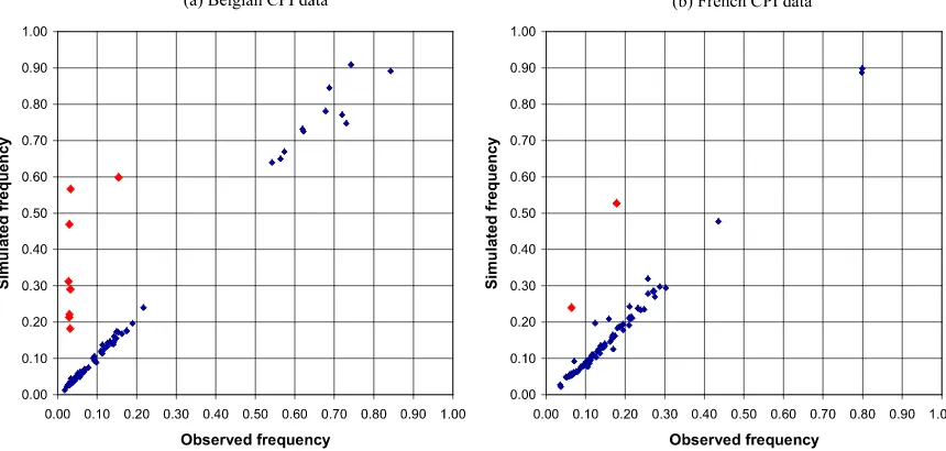
To evaluate the model’s goodness of fit, we simulated price trajectories for all products, using the estimated model parame-ters (details of this simulation exercise are provided in Section 5
Figure 1. Observed and simulated frequencies of price changes. The online version of this figure is in color.
of the online supplementary materials). The scatterplots of the realized and simulated frequencies for the 94 product categories in the Belgian CPI and the 88 product categories for the French CPI are presented in Figure1.
The complete set of results by individual product is pro-vided in Tables 5 and 6 of the online supplementary materi-als, along with a number of summary statistics, including the average number of price trajectories per month, the correlation coefficient offˆtwith the corresponding product category price
index, and the frequency and average size (in absolute terms) of price changes. As can be seen from Figure1, except for a small number of products (8 out of the 94 for the Belgian CPI and 2 out of 88 for the French CPI), the simulated frequency of price changes matches the observed ones quite closely. The excep-tions tended to be products with relatively rigid prices. These products are “dining room oak furniture,” “cup and saucer,” “parking spot in a garage,” “fabric for dress,” “wallet,” “small anorak,” “men’s T shirt,” and “hair spray 400 ml” in Belgium, and “classic lunch in a restaurant” and “pasta” in France. For
these 10 products, our simulations overestimate the frequency and underestimate the average size of price changes. In what follows, we exclude these products and focus on the remaining 172 products that seem to fit the observed price changes reason-ably well.
4.2 Characteristics of Price Changes by Product Categories
The main statistics regarding the price changes observed for these 172 products, grouped into six broad categories (energy, perishable food, nonperishable food, nondurable manufactured goods, durable manufactured goods, and services) are provided in Table1. These statistics show that the patterns of consumer price changes are essentially similar in Belgium and in France, and are in line with the previous empirical evidence regarding price changes in the Euro area (see, e.g.,Dhyne et al. 2006). Energy product prices are changed very frequently but by small amounts, whereas services exhibit small but quite infrequent
Table 1. Descriptive statistics by broad product categories—CPI weighted averages
Perishable Nonperishable Nondurable Durable
Energy food food goods goods Services
Belgium
Freq 0.723 0.315 0.127 0.145 0.056 0.041
|p| 0.039 0.139 0.102 0.083 0.072 0.056
% smallp 31% 34% 32% 33% 38% 36%
No. of products 3 23 12 15 18 15
France
Freq 0.799 0.247 0.204 0.124 0.134 0.077
|p| 0.022 0.119 0.064 0.166 0.083 0.047
% smallp 36% 50% 47% 41% 44% 43%
No. of products 2 13 11 31 13 16
NOTE: Freqis the observed frequency of price changes.|p|is the observed average absolute value of price changes. % small
pis, followingMidrigan(2011), the fraction of price changes of magnitude less than half of the average price change (in absolute value) in the product category.
price changes. Somewhere in between, the frequency and mag-nitude of price changes for food products are both quite high, whereas those for other manufactured goods are of lower fre-quency and magnitude. Clearly, there is a significant degree of heterogeneity in the price setting behavior across these prod-ucts.
It is also interesting that if we exclude energy products, then the ranking of the product categories by the frequency of price changes is the same as that by the average size of these price changes. All product categories also display a significant frac-tion of small price changes. It is difficult to explain both of these features with a standard(S,s)model in which the band of price inaction is fixed across outlets and products. Thus it is reasonable to expect that our more general specification of the (S,s)model, in which the band of inaction is allowed to vary across outlets and over time, could better fit the wide variety of outcomes observed across different products. This conjecture is supported by the additional empirical evidence provided in Section 6 of the online supplementary materials on the ability of alternative state-dependent pricing models to generate small price changes.
4.3 Parameter Estimates by Product Categories
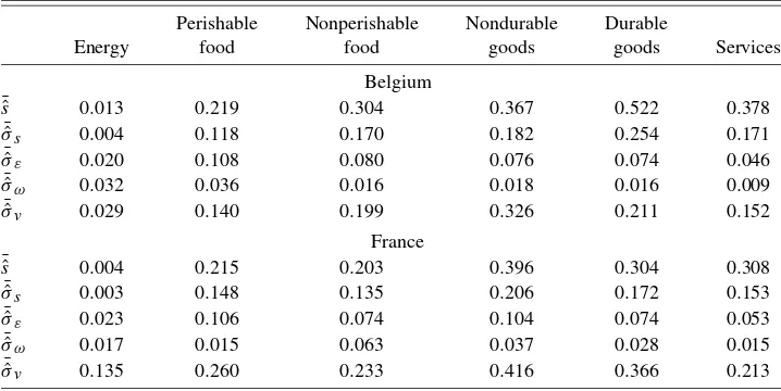
A summary of the ML estimates of the main parameters of interest is given in Table2. A full set of estimates by individ-ual commodities is provided by Tables 5 and 6 of the online supplementary materials. To compute σˆω2, the estimated vari-ance of common shocks, we assume thatft follows a general
autoregressive process possibly with a linear trend. Therefore, for each product category, we use the estimatesˆf1,fˆ2, . . . ,fˆT to
fit an AR(K)model, defined as
ˆ
ft=β0+β1t+ K
k=1
ρkfˆt−k+ωt, ωt∽iid(0, σω2),
where for each product category,Kis selected using the Akaike information criterion applied to autoregressions with the maxi-mum value ofKset to 12.
Not surprisingly, given the proximity of the price change characteristics in the two countries, the parameter estimates show similar qualitative patterns in France and Belgium. In-frequent and small price changes in the case of services are as-sociated with large estimates of inaction bands and relatively low estimates of shock volatilities. Indeed, wages are the most important cost component for the production of services, and their variations tend to be rather infrequent and limited (see, e.g., Heckel, Le Bihan, and Montornès2008). This explains in part why, despite the relatively large inaction band estimates obtained for services, service prices change by rather limited amounts; the magnitude of the variations in the underlying costs is indeed quite small.
Now consider the estimates for the energy prices, which tend to exhibit opposite characteristics to those of service prices. The estimated thresholds appear to be quite small. Moreover, the estimates of the variances of the shocks, although quite small in magnitude, are larger than the estimated mean thresholds, thus explaining the observed high frequency and small magnitude of price changes. Taken together, these results imply that energy prices are flexible.
Regarding the other categories of goods, it can be seen that the higher frequency of price changes for food products com-pared with manufactured products seems to stem from smaller inaction bands rather than from larger shocks. Also notewor-thy is the strong link between the mean inaction band,s,and its variability,σs; the correlation between the estimates of these
two parameters is 0.95 at the product level.Gautier and Le Bi-han (2011) explained why these two parameters are strongly positively linked. To explain the coexistence of small and large price changes, both parameters must take large values; that is, the variance ofsmust increase withsto allow the same propor-tion of small price changes when price changes are larger on average.
Overall, the larger the ¯ˆs(the weighted average estimate of the mean of the inaction band), the smaller the frequency of price changes. But the magnitude of shocks also plays a role in explaining these low frequencies.
Table 2. Parameter estimates by broad product categories—CPI weighted averages
Perishable Nonperishable Nondurable Durable
Energy food food goods goods Services
Belgium
¯ˆ
s 0.013 0.219 0.304 0.367 0.522 0.378
¯ˆ
σs 0.004 0.118 0.170 0.182 0.254 0.171
¯ˆ
σε 0.020 0.108 0.080 0.076 0.074 0.046
¯ˆ
σω 0.032 0.036 0.016 0.018 0.016 0.009
¯ˆ
σv 0.029 0.140 0.199 0.326 0.211 0.152
France
¯ˆ
s 0.004 0.215 0.203 0.396 0.304 0.308
¯ˆ
σs 0.003 0.148 0.135 0.206 0.172 0.153
¯ˆ
σε 0.023 0.106 0.074 0.104 0.074 0.053
¯ˆ
σω 0.017 0.015 0.063 0.037 0.028 0.015
¯ˆ
σv 0.135 0.260 0.233 0.416 0.366 0.213
NOTE: ¯ˆsis the average estimate of the mean of the price inaction band.σ¯ˆsis the average estimate of the standard deviation
of the price inaction band.σ¯ˆεis the average estimated standard deviation of the idiosyncratic component.σ¯ˆωis the average estimated standard deviation of the common shock.σ¯ˆvis the average estimated standard deviation of the outlet-specific shock.
All averages are weighted averages using the CPI weights of individual product categories and are computed over the individual estimates for the products in the specified product categories.
4.4 Common and Idiosyncratic Shocks
Now consider the estimates ofσωandσε(volatilities of com-mon and idiosyncratic shocks, respectively) summarized in Ta-ble 2. It is clear that for all product categories except energy products in Belgium, the weighted average estimates of σω (computed using the CPI weights and the individual product estimates within a given category) are much smaller than the weighted average estimates obtained forσε, suggesting that id-iosyncratic shocks generally may be more important than com-mon shocks. Of the 172 products under consideration,σˆε/σˆωis >1 for 165 products (84 in Belgium and 81 in France). This re-sult is in line with the conclusion ofGolosov and Lucas(2007), who found that price trajectories at the micro level are largely affected by idiosyncratic shocks.Nakamura(2008) also found that shocks common to all retailers represent only a small frac-tion of price changes (16%), and that promofrac-tions and sales are likely to explain the idiosyncratic price changes. However, it is worth recalling that in France and Belgium, sales periods are regulated and are then highly synchronized across outlets.
What can be inferred from these estimates about the respec-tive role of shocks and of adjustment costs in explaining the main characteristics of observed price changes? We know that the frequency and magnitude of price changes depend on the variance of shocks as well as ons(andσs), which in turn are
un-known functions of price adjustment costs and the shock vari-ances. To assess the relative importance of these parameters for the observed price changes, we ran a number of quadratic re-sponse surface regressions in which the price change character-istics were regressed on the estimates ofs,σs, σω,andσε, their squares, and their interactions. The idea was to isolate the ef-fects of common and idiosyncratic shocks, having purged out the influences of price inaction band and of its variability. We also considered includingσˆv in the analysis, but found its
ef-fects to be statistically insignificant, perhaps not surprisingly, becauseviare fixed over time, and they can have an influence
on price changes only through the nonlinear form of the(S,s) price function. In a linear price function, price changes do not depend onvi(and thus onσv).
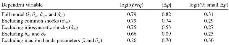
We ran these quadratic response surface regressions for all of the three price change characteristics discussed earlier, namely the frequency of the price changes (in log-odds ratio form), the magnitude of the price changes, and the fraction of small price changes (in log-odds ratio form). The results are summa-rized in Table3. For each price change characteristic, we report degrees-of-freedom adjustedR2 when all parameter estimates
were included (the “full model”), along with their various sub-sets.
The results of estimating these response surfaces are quite clear. The inaction band characteristics (sˆ and σˆs) strongly
contribute to explaining differences in the frequency of price changes. Excluding these estimates from the response surface for the frequencies of price changes leads to a sizeable de-crease in the adjusted R2. If we are ready to accept that a quadratic function like the one estimated here provides an ac-ceptable approximation to the unknown functions linking the frequency of price changes to adjustment costs and the vari-ances of shocks through the inaction band parameters, then this result demonstrates a strong heterogeneity of adjustment costs across goods and their importance for explaining the frequency of price changes.
On the other hand, the magnitude of price changes strongly depends on the size of the shocks, with the idiosyncratic shocks playing a major role in this respect. These can be interpreted as representing the decisions of outlets to make limited-time promotions (seeHosken and Reiffen 2004orNakamura 2008 for explanations of why common shocks cannot explain the ob-served consumer price changes at the outlet level). However, this might not be the appropriate explanation here, because sale periods were strictly regulated during the period covered by our data, and other kinds of promotions do not seem to be that fre-quent (Baudry et al. 2007). Given the nature of the relationships between producers and retailers, these idiosyncratic changes might indeed result from changes in outlet-specific wholesale prices (see, e.g., Réquillart, Simioni, and Varela-Irimia2009). Section 6 of the online supplementary materials shows that our model, by allowing the band of inaction to vary over time and across outlets, is an improvement over the standard(S,s)model in its ability to capture the frequency of small price changes, but nonetheless is still unable to fully reproduce the observed fre-quency of small price changes. Further research in this area is clearly needed.
5. CONCLUSION
In this article we specify and estimate a state-dependent(S,s) type model with stochastic thresholds where the unobserved op-timal price targeted by outlets is decomposed into four compo-nents: a common factor, an idiosyncratic component, a random outlet-specific effect, and a fourth component associated with the observed characteristics of the outlet. This setup involves modeling of the price change as a nonlinear dynamic panel
Table 3. Assessing the importance of shocks and inaction band parameters on price change characteristics
Dependent variable logit(Freq) |p| logit(% smallp)
Full model (ˆs,σˆs,σˆω, andσˆε) 0.79 0.82 0.31
Excluding common shocks (σˆω) 0.79 0.74 0.29
Excluding idiosyncratic shocks (σˆε) 0.75 0.53 0.27
Excludingσˆωandσˆε 0.66 0.09 0.25
Excluding inaction bands parameters (ˆsandσˆs) 0.26 0.70 0.30
NOTE: The reported figures are the adjustedR2of quadratic response surface regressions for the specified model. logit(y)=log(y/(1−
y)).Freqis the observed frequency of price changes.|p|is the observed average absolute value of price changes. % smallpis, following
Midrigan(2011), the fraction of price changes of magnitude less than half of the average price change (in absolute value) in the product category.
model with unobserved common effects. The(S,s)model that we consider thus represents a nonlinear extension of the factor models used extensively in the empirical finance and macroe-conomic literature. The model extends the work ofHosken and Reiffen (2004) and Nakamura (2008) in that it explicitly ac-counts for the existence of periods of price stability between two price changes in estimating the common component of the price change. Using two large datasets comprising consumer price records used to compute the CPI in Belgium and France, this model is estimated for 182 goods and services covering a very wide range of consumer products.
Our estimation results confirm the pervasive degree of het-erogeneity in price behavior across products. The frequency of price changes appears to depend more strongly on the charac-teristics of the band of inaction (its average width as well as its variance) than on the variability of shocks to the optimal price. However, the latter are by far the most important drivers of the magnitude of price changes, with the idiosyncratic shocks play-ing a major role in this respect. Explainplay-ing small price changes appears to be more difficult. However, our model improves on models with a fixed band of price inaction, asymmetric inac-tion bounds, or seasonal adjustment bounds in replicating the occurrence of small price changes.
SUPPLEMENTARY MATERIALS
Data sources, derivations and proofs, Monte Carlo simula-tions, and additional results: A document containing sup-plementary materials for this article covers data sources, mathematical derivations and proofs, Monte Carlo simula-tions that shed light on the properties of the proposed es-timation procedures, reports product specific estimates, and provides additional empirical results on the ability of state dependent pricing models to generate small price changes. (Supplements.pdf)
ACKNOWLEDGMENTS
The views expressed are those of the authors and do not nec-essarily reflect the views of the National Bank of Belgium or of the Banque de France. The authors thank the INS-NIS (Bel-gium) and the INSEE (France) for providing the micro price data and Luc Aucremanne, Jeffrey Campbell, Vassilis Hajivas-siliou, Cheng Hsiao, Jerzy Konieczny, Hervé Le Bihan, Daniel Levy, and Rafaël Wouters for their comments on early drafts. Constructive suggestions and criticisms from an associate ed-itor and two anonymous referees are also gratefully acknowl-edged.
[Received March 2009. Revised July 2010.]
REFERENCES
Aucremanne, L., and Dhyne, E. (2004), “How Frequently Do Prices Change? Evidence Based on the Micro Data Underlying the Belgian CPI,” Working Paper 331, ECB. [531,535]
(2005), “Time-Dependent versus State-Dependent Pricing: A Panel Data Approach to the Determinants of Belgian Consumer Price Changes,” Working Paper 462, ECB. [531]
Bacon, R. W. (1991), “Rockets and Feathers: The Asymmetric Speed of Adjust-ment of UK Retail Gasoline Prices to Cost Changes,”Energy Economics, 13 (3), 211–218. [529]
Bai, J., and Ng, S. (2002), “Determining the Number of Factors in Approximate Factor Models,”Econometrica, 70 (1), 191–221. [530]
(2006), “Evaluating Latent and Observed Factors in Macroeconomics and Finance,”Journal of Econometrics, 131, 507–537. [530]
Baudry, L., Le Bihan, H., Sevestre, P., and Tarrieu, S. (2007), “What Do Thir-teen Million Price Records Have to Say About Consumer Price Rigidity?” Oxford Bulletin of Economics and Statistics, 69 (2), 139–183. [535,538] Bils, M., and Klenow, P. (2004), “Some Evidence on the Importance of Sticky
Prices,”Journal of Political Economy, 112 (5), 947–985. [529,530] Blinder, A. S., Canetti, E. R. D., Lebow, D. E., and Rudd, J. B. (1998),Asking
About Prices: A New Approach to Undertsanding Price Stickiness, New York: Russel Sage Foundation. [530,531]
Borenstein, S., Cameron, A. C., and Gilbert, R. (1997), “Do Gasoline Prices Respond Asymmetrically to Crude Oil Price Changes?”Quarterly Journal of Economics, 112 (1), 305–339. [529]
Caballero, R., and Engel, E. (1999), “Explaining Investment Dynamics in U.S. Manufacturing: A Generalized (S,s) Approach,” Econometrica, 67 (4), 783–826. [530]
(2007), “Price Stickiness inSsModels: New Interpretations of Old Results,”Journal of Monetary Economics, 54 (Supplement 1), 100–121. [531]
Calvo, G. (1983), “Staggered Prices in a Utility-Maximizing Framework,” Jour-nal of Monetary Economics, 12, 383–398. [530]
Campbell, J. R., and Eden, B. (2005), “Rigid Prices: Evidence From U.S. Scan-ner Data,” Working Paper 05-08, Federal Reserve Bank of Chicago. [531] Cecchetti, S. G. (1986), “The Frequency of Price Adjustments: A Study of the
Newsstand Price of Magazines,”Journal of Econometrics, 31 (3), 255–274. [529-531]
Connor, G., and Korajczyk, R. A. (1986), “Performance Measurement With the Arbitrage Pricing Theory,”Journal of Financial Economics, 15, 373–394. [530]
(1988), “Risk and Return in an Equilibrium APT: Application of a New Test Methodology,”Journal of Financial Economics, 21, 255–289. [530] Cornille, D., and Dossche, M. (2008), “Some Evidence on the Adjustment of
Producer Prices,”Scandinavian Journal of Economics, 110 (3), 489–518. [529]
Costain, J., and Nakov, A. (2011), “Price Adjustments in a General Model of State-Dependent Pricing,”Journal of Money, Credit and Banking, 43 (2–3), 385–406. [530]
Davis, M., and Hamilton, J. (2004), “Why Are Prices Sticky? The Dynamics of Wholesale Gasoline Prices,”Journal of Money, Credit and Banking, 36 (1), 17–38. [529,530]
Dhyne, E., Álvarez, L. J., Le Bihan, H., Veronese, G., Dias, D., Hoffmann, J., Jonker, N., Lünnemann, P., Rumler, F., and Vilmunen, J. (2006), “Price Changes in the Euro Area and the United States: Some Facts From Individ-ual Consumer Price Data,”Journal of Economic Perspective, 20 (2), 171– 192. [529,530,536]
Dixit, A. (1991), “Analytical Approximations in Models of Hysteresis,”Review of Economic Studies, 58 (1), 141–151. [531]
Dotsey, M., King, R. G., and Wolman, A. L. (1999), “State-Dependent Pricing and the General Equilibrium Dynamics of Money and Output,”Quarterly Journal of Economics, 114 (2), 655–690. [530]
Dutta, S., Bergen, M., and Levy, D. (2002), “Price Flexibility in Channels of Distribution: Evidence From Scanner Data,”Journal of Economic Dynam-ics and Control, 26 (11), 1845–1900. [529,530]
Eichenbaum, M., and Fisher, J. D. M. (2007), “Estimating the Frequency of Price Re-Optimization in Calvo-Style Models,”Journal of Monetary Eco-nomics, 54 (7), 2032–2047. [530]
Forni, M., Hallin, M., Lippi, M., and Reichlin, L. (2000), “The Generalised Dy-namic Factor Model: Identification and Estimation,”Review of Economics and Statistics, 82 (4), 540–554. [530]
Fougère, D., Gautier, E., and Le Bihan, H. (2010), “Restaurant Prices and the Minimum Wage,”Journal of Money, Credit and Banking, 42 (7), 1199– 1234. [530,531]
Fougère, D., Le Bihan, H., and Sevestre, P. (2007), “Heterogeneity in Price Stickiness: A Microeconometric Investigation,”Journal of Business & Eco-nomic Statistics, 25 (3), 247–264. [530,531]
Gagnon, E. (2009), “Price Setting During Low and High Inflation: Evidence From Mexico,”Quarterly Journal of Economics, 124 (3), 1221–1263. [530] Gautier, E., and Le Bihan, H. (2011), “Time-Varying (S,s) Band Models: Prop-erties and Interpretation,”Journal of Economic Dynamics and Control, 35 (3), 394–412. [537]
Gertler, M., and Leahy, J. (2006), “A Phillips Curve With anSsFoundation,” Working Paper 11971, NBER. [531]
Golosov, M., and Lucas, R. E. (2007), “Menu Costs and Phillips Curves,” Jour-nal of Political Economy, 115 (2), 171–199. [529,538]
Hansen, P. S. (1999), “Frequent Price Changes Under Menu Costs,”Journal of Economic Dynamics and Control, 23, 1065–1076. [531]
Heckel, T., Le Bihan, H., and Montornès, J. (2008), “Sticky Wages: Evidence From Quarterly Microeconomic Data,” Working Paper 893, ECB. [537] Hosken, D. S., and Reiffen, D. (2004), “Patterns of Retail Price Variation,”
RAND Journal of Economics, 35 (1), 128–146. [529-531,538,539] Kashyap, A. K. (1995), “Sticky Prices: New Evidence From Retail Catalogs,”
Quarterly Journal of Economics, 110 (1), 245–274. [529]
Klenow, P., and Kryvtsov, O. (2008), “State-Dependent or Time-Dependent Pricing: Does It Matter for Recent U.S. Inflation?”Quarterly Journal of Economics, 123 (3), 863–904. [529,531]
Klenow, P., and Willis, J. (2007), “Sticky Information and Sticky Prices,” Jour-nal of Monetary Economics, 54, 79–99. [530]
Lach, S., and Tsiddon, D. (1992), “The Behaviour of Prices and Inflation: An Empirical Analysis of Disaggregated Price Data,”Journal of Political Econ-omy, 100 (2), 349–389. [529,530]
Levy, D., Bergen, M., Dutta, S., and Venables, R. (1997), “The Magnitude of Menu Costs: Direct Evidence From Large U.S. Supermarket Chains,” Quar-terly Journal of Economics, 112 (3), 791–825. [531]
Loupias, C., and Sevestre, P. (2010), “Costs, Demand and Producer Price Changes,” Working Paper 273, Banque de France. [529]
Mankiw, G., and Reis, R. (2006), “Pervasive Stickyness,”American Economic Review, 96 (2), 164–169. [530]
Midrigan, V. (2011), “Menu Costs, Multiproduct Firms, and Aggregate Fluctu-ations,”Econometrica, 79 (4), 1139–1180. [536,538]
Nakamura, E. (2008), “Pass-Through in Retail and Wholesale,”American Eco-nomic Review, 98 (2), 430–437. [529-531,535,538,539]
Nakamura, E., and Steinsson, J. (2008), “Five Facts About Prices: A Reeval-uation of Menu Cost Models,”Quarterly Journal of Economics, 123 (4), 1415–1464. [529,530]
Peltzman, S. (2000), “Prices Rise Faster Than They Fall,”Journal of Political Economy, 108 (3), 466–502. [530]
Pesaran, M. H. (2006), “Estimation and Inference in Large Heterogeneous Pan-els With a Multifactor Error Structure,”Econometrica, 74 (4), 967–1012. [533]
Ratfai, A. (2006), “Linking Individual and Aggregate Price Changes,”Journal of Money, Credit and Banking, 38 (8), 2199–2224. [529-531,535] Réquillart, V., Simioni, M., and Varela-Irimia, X. L. (2009), “Imperfect
Com-petition in the Fresh Tomato Industry,” mimeo, Toulouse School of Eco-nomics. [538]
Rosett, R. N. (1959), “A Statistical Model of Frictions in Economics,” Econo-metrica, 27 (2), 263–267. [531]
Sheshinski, E., and Weiss, Y. (1977), “Inflation and Costs of Adjustment,” Re-view of Economic Studies, 44 (2), 281–303. [530,531]
(1983), “Optimal Pricing Policy Under Stochastic Inflation,”Review of Economic Studies, 51 (3), 513–529. [531]
Sims, C. (2003), “Implications of Rational Inattention,”Journal of Monetary Economics, 50 (3), 665–690. [530]
Stock, J. H., and Watson, M. W. (1998), “Diffusion Indexes,” Working Pa-per 6702, NBER. [530]
(2002), “Macroeconomic Forecasting Using Diffusion Indexes,” Jour-nal of Business & Economic Statistics, 20 (2), 147–162. [530]
Tsiddon, D. (1993), “The (Mis)Behaviour of the Price Level,”Review of Eco-nomic Studies, 60 (4), 889–902. [531]
Vermeulen, P., Dias, D., Dossche, M., Gautier, E., Hernando, I., Sabbatini, R., and Stahl, H. (2007), “Price Setting in the Euro Area: Some Stylised Facts From Individual Producer Price Data,” Working Paper 727, ECB. [529] Willis, J. (2006), “Magazine Price Revisited,”Journal of Applied Econometrics,
21, 337–344. [531]
Woodford, M. (2009), “Information-Constrained State-Dependent Pricing,” Journal of Monetary Economics, 56 (S1), 100–124. [530]
Zbaracki, M., Ritson, M., Levy, D., Dutta, S., and Bergen, M. (2004), “Man-agerial and Customer Costs of Price Adjustment: Direct Evidence From Industrial Markets,”Review of Economics and Statistics, 86 (2), 514–533. [531]