in PROBABILITY
A LIMIT LAW FOR THE ROOT VALUE OF MINIMAX
TREES
T ¨AMUR ALI KHAN
Department of Mathematics and Computer Science Johann Wolfgang Goethe Universit¨at
60054 Frankfurt am Main Germany
email: [email protected]
LUC DEVROYE1
School of Computer Science McGill University
Montreal, H3A 2K6 Canada
email: [email protected]
RALPH NEININGER2
Department of Mathematics and Computer Science Johann Wolfgang Goethe Universit¨at
60054 Frankfurt am Main Germany
email: [email protected]
Submitted 22 November 2005, accepted in final form 16 December 2005 AMS 2000 Subject classification: 60F05, 68Q25, 60E05, 68T20.
Keywords: Minimax Tree, Limit Law, Weak Convergence, Analysis of Algorithms, Gametree.
Abstract
We consider minimax trees with independent, identically distributed leaf values that have a continuous distribution functionFV being strictly increasing on the range where 0< FV <1.
It was shown by Pearl that the root value of such trees converges to a deterministic limit in probability without any scaling. We show that after normalization we have convergence in distribution to a nondegenerate limit random variable.
1
Introduction and result
We study trees related to the analysis of game-searching methods for two-person perfect in-formation games like Chess or Go. In these games two players A and B start with an initial
1RESEARCH SUPPORTED BY NSERC GRANT 3456 AND BY A JAMES MCGILL FELLOWSHIP.
2RESEARCH SUPPORTED BY AN EMMY NOETHER FELLOWSHIP OF THE DFG.
position and take alternate turns, choosing each time amongd≥2 possible moves. A terminal position is reached after 2k,k≥0, moves. The terminal position does not necessarily termi-nate the game, but instead it termitermi-nates the horizon of a player or machine searching for best possible moves. One would like to assign a value to each position that indicates the chances of each player winning the game when starting from that position. Although, assuming best possible moves of both players, it is deterministic how the game terminates, the horizon 2k
of players or machines is usually limited so that they cannot plan their moves up to the very end of the game. To overcome this problem one assigns valuesV to terminal positions, where large values ofV indicate that the position favors player A, small values favor player B. Given the values of alln=d2k terminal nodes one can search for best possible moves for the starting
position and calculate its value.
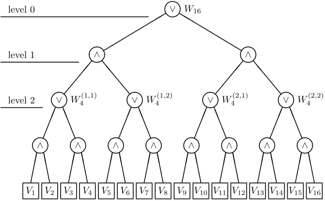
The possible moves and its terminal positions can be represented in a rooted tree with fixed branching degree d≥2 and height 2k, k≥0. Leaves are assigned random valuesV1, . . . , Vn,
Figure 1: A minimax tree with branching degree 2 and height 4.
These trees are called minimax trees. The value of a node is given as the value of the operator labeled at that node applied to the values of its children. This corresponds to player A always choosing the move with maximal value, player B always choosing a minimal value move. Thus fromV1, . . . , Vn one could first calculate the values of all nodes on level 2k−1 and successively
determine the values on higher levels leading finally the root’s value. The most popular algorithm for finding the leaf whose value trickles up to the root (which corresponds to the best moves when two intelligent players are playing) is alpha-beta pruning. Analysis of this algorithm for various models is given in Knuth and Moore [4], see also Zhang [11].
Minimax trees whereV1, . . . , Vnonly take the values 0 and 1 are also known as AND/OR trees
trees was given in Snir [10]. For probabilistic analysis of Snir’s algorithm see Saks and Wigder-son [9], Karp and Zhang [3], and Ali Khan and Neininger [1].
In this paper we are not concerned with the complexity of algorithms to determine the root’s value of minimax trees. We study the valueWn of the root itself asymptotically ask→ ∞.
We consider Pearl’s model where the leaves’ valuesV1, . . . , Vn are independent and identically
distributed random variables with a distributionL(V) having a distribution functionFV(x) =
P(V ≤x) that is continuous and strictly increasing on the range, where 0< FV <1, see Pearl [8]. For an alternative incremental model, see Nau [5, 6, 7] and the analysis in Devroye and Kamoun [2].
Pearl [8] showed for his model that Wn converges, without any scaling, in probability to a
deterministic limitqV asn=d2k tends to infinity,
Wn −→P qV, (k→ ∞),
and characterized the value ofqV.
In this paper we derive a limit law forWn after appropriate rescaling. We denote the
distri-bution function of Wn byFn. Note that this is defined for all n=d2k with k∈N0 and that
we haveF1=FV. Moreover, fork≥1, we haveFn=f◦Fn/d2 with
f(x) =¡
1−(1−x)d¢d
, x∈[0,1]. (1)
This is implied by the recursive structure of the tree: The values of thed2nodes on level 2 are
independent and identically distributed with distribution L(Wn/d2). We denote these values byWn/d(i,j)2 withi, j= 1, . . . , d, see Figure 1 for the cased= 2. Hence, by independence we have
Fn(x) =P
à d
_
i=1 d
^
j=1
Wn/d(i,j)2≤x !
= µ
1−³1−P³W(i,j)
n/d2 ≤x ´´d¶d
=f(Fn/d2(x)).
Function f has the fixed points 0 and 1 and there is a unique fixed point in the open unit interval (0,1) that we denote byq, cf. Lemma 2 below. It was shown by Pearl [8] that we have
qV =FV−1(q).
We denote the slope off in qbyξ=f′(q). Then the following limit law holds.
Theorem 1 With FV, q and ξ as above and d ≥ 2 we have the following convergence in
distribution for the valueWn of the minimax tree in Pearl’s model. Withα= log(ξ)/log(d2)∈
(0,1),
nα(FV(Wn)−q)
L
−→W, k→ ∞. (2)
The random variable W does not depend upon L(V), has a continuous distribution function
FW with0< FW <1,FW(0) =q and
FW(x) =f(FW(x/ξ)), x∈R, (3)
0 0.1 0.2 0.3 0.4 0.5 0.6 0.7 0.8 0.9 1.0 1.1 1.2 -0.1
-0.2 -0.3 -0.4 -0.5 -0.6 -0.7 -0.8 -0.9 -1.0
0 0.1 0.2 0.3 0.4 0.5 0.6 0.7 0.8 0.9 1.0
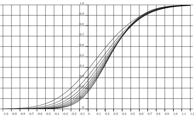
Figure 2: Approximations of the limit distribution function FW for d= 2, . . . ,10. They can
be distinguished by FW(0) = qd being decreasing in d. As approximations the functions g6
defined in (7) are plotted.
An approximation of the limit distribution function FW is plotted in Figure 2 for the cases
d= 2, . . . ,10.
Note that the transformation FV(Wn) ofWnin (2) allows to rewrite FV(Wn) as follows: The
random variable FV(Wn) is distributed as the root’s valueWn′ of a minimax tree with same
branching degree and height where the independent, identically distributed leaves now have distribution L(V′) =L(F
V(V)) = unif[0,1], the uniform distribution on [0,1]. Hence without
loss of generality one may assume thatL(V) = unif[0,1].
The rest of this note contains a proof of Theorem 1. We first collect some properties of f in section 2, since later on the recurrence relationFn =f◦Fn/d2 is exploited. Section 3 contains the proof of Theorem 1.
2
Technical preliminaries
We collect some properties of the functionf defined in (1).
Lemma 2 There is a unique q∈(0,1) withf(q) =q. We have ξ=f′(q) =d2q2/(1−q)2∈
(1, d2). Furthermore, forz:= 1−1/(d+ 1)1/d, we have
f′′(x)
>0 for0< x < z,
= 0 forx=z, <0 forz < x <1.
(4)
Proof. For 0< x <1 we have
f′(x) =d2(1−x)d−1(1−(1−x)d)d−1, (5)
f′′(x) =d2(d−1)(1−x)d−2(1−(1−x)d)d−2((d+ 1)(1−x)d−1). (6)
From this the (in-)equalities (4) follow with z = zd = 1−1/(d+ 1)1/d. For existence and
uniqueness of the fixed pointqoff in (0,1) we first show: Claim: f(zd)−zd>0 for alld≥2.
The claim follows ford= 2,3 by explicit calculation. Furthermore we havef(zd) = (1−1/(d+
1))d↓1/e asd→ ∞, hencef(z
d)≥1/e for alld≥4. It is easily seen thatzd is decreasing in
d, thuszd≤z4for alld≥4. Consequently, for alld≥4
f(zd)−zd≥
1
e−z4=
1
e + 1−
1 51/4 >0,
which implies the claim.
Since f(0) = f′(0) = 0, there exists 0 < ε < z
d with f(x)−x < 0 for all 0 < x ≤ ε.
Together with the previous claim, continuity and the intermediate value theorem we obtain a fixed point off in (ε, zd). We denote byq=qd the smallest fixed point off in (0, zd), which
exists by continuity and satisfies q > ε > 0. Then we have f(x)< x for all x∈ (0, q). For
x ∈ (q, z) we have f(x)> x by convexity of f on [0, z]: Otherwise there was an x∈ (q, z) with f(x)≤x. For arbitrary y ∈(0, q), andλ∈ (0,1) withq =λy+ (1−λ)xthis implied
f(q)≤λf(y) + (1−λ)f(x)< λy+ (1−λ)x=q, a contradiction. Similarly, concavity off on [z,1] impliesf(x)> xfor allx∈(z,1): For all suchxthere is aλ∈(0,1) withx=λz+(1−λ)1 thusf(x)≥λf(z) + (1−λ)f(1)> λz+ (1−λ)1 =x. Altogether,q is the unique fixed point off in (0,1).
It remains to prove that ξ = ξd = f′(q) = d2q2/(1−q)2 ∈ (1, d2). For this note that the
functionud: [0,1]→[0,1],x7→(1−x)d, has a unique fixed point in (0,1). Sincef =ud◦ud
this fixed point must beq=qd, hence we obtain the relationq= (1−q)d. Using this relation in
(5) impliesξ=f′(q) =d2q2/(1−q)2. Moreover, sinceu
d′ ≤udfor all 2≤d≤d′ the sequence
(qd)d≥2 is decreasing. Thusqd≤q2= (3−
√
5)/2<1/2 for alld≥2, hence ξd< d2. Finally,
q= (1−q)d,f′′(q)>0 and the representation (6) implyq >1/(d+ 1), henceq/(1−q)>1/d
andξ > d2/d2= 1.
✷
In the following, it is convenient to extend functionf defined in (1) to the real line by setting
f(x) = 0 forx <0 andf(x) = 1 forx >1. We denote the iterations off byfk=f◦fk−1 for
k≥1 andf0(x) =xfor all x∈R. In particular, we have f1 =f. Using Fn =f◦Fn/d2 we obtain forn=d2k that Fn =fk◦F1=fk◦FV.
For the quantitiesnα(F
V(Wn)−q) of Theorem 1 we obtain with the relationnα=ξk
P(nα(FV(Wn)−q)≤x) =P µ
Wn≤FV−1
µ
q+ x
ξk
¶¶
=Fn◦FV−1
µ
q+ x
ξk
=fk
µ
q+ x
ξk
.
Thus, the functionsgk :R→Rdefined by
gk(x) =fk
µ
q+ x
ξk
are the distribution functions of nα(F
V(Wn)−q) forn=d2k,k≥0.
Subsequently we will need bounds forgk valid locally aroundx= 0 and uniformly ink≥0.
Lemma 3 Denoteh1(x) :=q+xandh2(x) :=q+x+cx2forx∈Rwithc:= 1+f′′(q)/(2ξ(ξ−
Thus, the induction proof is completed by showing that for someε >0 we have
f
for allxin a bounded neighborhood of 0. We have
1
3
Proof of the theorem
We proof the claims of Theorem 1.
Convergence in distribution: We show thatnα(F
V(Wn)−q) converges in distribution by
showing that its distribution functions gk, n = d2k, convergence pointwise to a distribution
Fixx∈R. Since q < z andf′(q) =ξ >1 there isk0(x) such that 0< q+x/ξk < z, for all
and, sincefk−1 is monotone increasing,
gk(x) =fk gent. We denote its limit by
g(x) := lim
k→∞gk(x), x∈
R.
Sincegk is nondecreasing for all k≥1 its limitg is a nondecreasing function. Sincegk(0) =
fk(q) =qfor everyk≥0, we haveg(0) =q. Continuity off andgk(x) =f(gk−1(x/ξ)) yields,
withk→ ∞, the functional equationg(x) =f(g(x/ξ)).
Monotonicity ofgand 0≤g≤1 imply that limx→∞g(x) and limx→−∞g(x) exist. Continuity
off andξ >0 yield with the functional equation forg that
lim
Hence, both limits are fixed points of f. Lemma 3 and convergence ofgk yield, with εas in
Lemma,
random variableW with distribution functionFW = ¯g.
Note that up to now we only knowg(x) = ¯g(x) for continuity pointsxof ¯g. (We will see below thatg is continuous, henceg(x) = ¯g(x) =FW(x) for allx∈R.) ✷
Continuity of g: We show thatgis continuous in allx∈Rby distinguishing the three cases
x <0, x= 0 and x >0. Note that for all x∈R it is sufficient to show that there exists a Case x <0: The chain rule and induction imply
For x≤0 we have fi(q+x/ξk)≤q. Sincef′ is monotone increasing on (−∞, q] we obtain
g′
k(x)≤(f
′(q)/ξ)k = 1 for allx≤0 andk≥0. Hence, for allx <0 we have (10) withC= 1.
Case x= 0: By Lemma 3 and ¯g(x) =g(x) for allx <0 we obtain P(W <0) = lim
ℓ→∞
P µ
W ≤ −1ℓ 
= lim
ℓ→∞g¯
µ −1ℓ
¶ = lim
ℓ→∞g
µ −1ℓ
≥ lim
ℓ→∞h1
µ −1ℓ
=q. (12)
Since g is a monotone function it has at most countably many discontinuity points. Hence there exists a sequence (xℓ)ℓ≥1 of continuity points ofg withxℓ↓0. Then, with Lemma 3 we
obtain
P(W >0) = 1− lim
ℓ→∞
P(W ≤xℓ) = 1− lim
ℓ→∞¯g(xℓ) = 1−ℓlim→∞g(xℓ)
≥1− lim
ℓ→∞h2(xℓ) = 1−q. (13)
Inequalities (12) and (13) together implyP(W = 0) = 0, hencegis continuous inx= 0. Since we have g(0) =q this impliesFW(0) =g(0) =q.
Case x >0: We first show the following assertion: Claim: There exists a 0< ε≤z−q such thatg′
k is a monotone increasing function on [0, ε]
for allk≥0.
The claim is shown as follows: Since g is continuous in 0 and g(0) = q < z there exists a 0< ε < z−qwithg(y)≤zfor all 0≤y≤ε. By monotonicity of thefi, we have for allk≥0,
0≤i≤kand 0< y′ < y
≤ε
fi(q+y′/ξk)≤fi(q+y/ξk)≤fi(q+y/ξi) =gi(y)≤g(y)≤z.
For the second last inequality in the latter display note that (gi)i≥0is increasing on (−∞, z−q),
cf. (9). Since f′ is monotone increasing on (−∞, z] this yields
f′(f
i(q+y′/ξk))≤f′(fi(q+y/ξk)),
thus by (11) we obtaing′
k(y′)≤gk′(y) which implies the claim.
Now, assumeg is discontinuous in some x′>0. Letεbe as in the previous claim. Note that
all the pointsx′/ξk,k≥0, are discontinuities ofgby the functional equationg(x) =f(g(x/ξ))
and continuity off. Hence there exists a discontinuity 0< x < ε/2 ofg. By (10), we have for all 0< δ <(ε/2−x)∧x,
supng′
k(y)
¯ ¯
¯y:|y−x|< δ, k≥0 o
=∞. (14)
Fix such aδ. By (14) and the claim we haveg′
m(x+δ)≥4/ε for a sufficiently largem. Now,
the claim implies g′
m(y)≥4/εfor ally∈[ε/2, ε]. Then,
gm(ε)−gm(ε/2) =
Z ε
ε/2
g′
m(y)dy≥
Z ε
ε/2
4
εdy= 2.
This is a contradiction, since gmis a distribution function. ✷
0<FW<1: Assume thatFW(x) =g(x)∈ {0,1} for somex∈R. Theng(x/ξk) =g(x) for
allk≥0. Hence by continuity ofg, we obtaing(0)∈ {0,1}. Sinceg(0) =q∈(0,1) this is a
Acknowledgment
We are grateful to Lars Kauffmann for performing simulations which helped finding the correct scaling in Theorem 1. We thank Gerold Alsmeyer and Matthias Meiners for sharing their knowledge aboutL(W) with us. We also thank the referee for helpful comments.
References
[1] Ali Khan, T. and Neininger, R. Probabilistic analysis for randomized game tree evaluation. Mathematics and computer science. III, 163–174, Trends Math.,Birkh¨auser, Basel, 2004. [2] Devroye, L. and Kamoun, O. Random minimax game trees. Random discrete structures
(Minneapolis, MN, 1993), 55–80, IMA Vol. Math. Appl., 76,Springer, New York, 1996 [3] Karp, R. M. and Zhang, Y. Bounded branching process and AND/OR tree evaluation.
Random Structures Algorithms 7(1995), 97–116.
[4] Knuth, D. E. and Moore, R. W. An analysis of alpha-beta pruning.Artificial Intelligence 6 (1975), 293–326.
[5] Nau, D. S. The last player theorem.Artificial Intelligence 18(1982), 53–65.
[6] Nau, D. S. An investigation of the causes of pathology in games.Artificial Intelligence 19 (1982), 257–278.
[7] Nau, D. S. Pathology on game trees revisited, and an alternative to minimaxing. (English) Artificial Intelligence 21(1983), 221–244 (1983).
[8] Pearl, J. Asymptotic properties of minimax trees in game-searching procedures.Aritificial Intelligence 14(1980), 113–126.
[9] Saks, M. and Wigderson, A. Probabilistic boolean decision trees and the complexity of evaluating game trees. Proceedings of the 27th Annual IEEE Symposium on Foundations of Computer Science, 29–38, Toronto, Ontario, 1986.
[10] Snir, M. Lower bounds on probabilistic linear decision trees. Theor. Comput. Sci. 38 (1985), 69-82.