ELECTRONIC
COMMUNICATIONS in PROBABILITY
CONNECTED ALLOCATION TO POISSON POINTS IN
R
2MAXIM KRIKUN
Institut ´Elie Cartan, Universit´e Henri Poincar´e, BP 239, 54506 VANDOEUVRE-LES-NANCY CEDEX - France
email: [email protected]
Submitted February 14 2007, accepted in final form April 20 2007 AMS 2000 Subject classification: 60D05
Keywords: Poisson process, Riemann map
Abstract
This note answers one question in [1], concerning the connected allocation for the Poisson process in R2
. The proposed solution makes use of the Riemann map from the plane minus the minimal spanning forest of the Poisson point process to the halfplane. A picture of a numerically simulated example is included.
1
The problem
LetX ⊂Rdbe a discrete set. We call the elements ofXcenters, the elements ofRd–sites, and we writeLfor the Lebesgue measure inR2
. AnallocationofRd toX withappetiteα∈[0,∞]
One particular question we’re interested in is the following [1]: Is there a translation-equivariant allocation for the Poisson process of unit intensity in the critical two-dimensional case (d= 2 andα= 1), in which every territory is connected? The goal of the present note is to describe one such allocation. Note: for a far more general approach to this question ind≥3 see [3].
2
Construction of a connected allocation
LetX be a realization of Poisson process (of intensity 1) inR2 .
Let theminimal spanning forestT be the union of edgese= (x, y),x, y ∈X, such that there is no path fromxtoy in the complete graph onX with all edges strictly shorter thane(see [4] for other definitions and references on the subject).
For a 2-dimensional Poisson process Alexander [2] proved thatTis a.s. a tree with one topologi-cal end (a topologitopologi-cal end in a graph is a class of equivalence of semi-infinite paths modulo finite
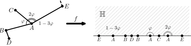
symmetric difference). Thus the domainD=R2
\T is simply connected, and by the Riemann mapping theorem can be mapped conformally to the upper half-planeH={z∈C:ℑ(z)>0}.
Moreover, we can choose such a mapping f which also sends infinity to infinity. (Note that any two such functions differ by a conformal automorphism ofHwhich invariates infinity, i.e.
by an affine mappingz→az+b,a, b∈R,a6= 0).
The mappingf cannot be extended unambiguously toT. Instead, consider the inverse mapping
g=f−1
from the open halfplane toD, then extendgto the real axis by continuity, obtaining a surjectiong:H→R2
. Some points ofX may have more than one preimage underg, more exactly, a point has as many preimages as it’s degree inT. For those points we’ll have to split their appetite between these preimages in some way, e.g. proportionally to the angle of the corresponding sector. Let (x′
n, α′n) be the resulting points and appetites. In the following we call the countable set{(x′
Figure 1: The image ofX underf; the unit appetite of the centerAis split into three unequal parts.
Now consider the followingstable allocation procedure(see Appendix II for a formal definition):
• Each center starts growing a ball centered in it. All the balls grow simultaneously, at the same linear speed.
• Each center claims the sites captured by it’s ball, unless the site was claimed earlier by some other center.
• Once the center becomes sated (the measure of it’s territory reaches it’s appetite), the ball stops growing.
Note that from our choice of function f it follows that the set {x′
n, n ∈ Z} is locally finite (i.e. has no accumulation point other than infinity), so the stable allocation procedure is well defined.
Applying this procedure to the image ofX under f in the half-planeH, with respect to the
Euclidean metric in H and the image λ of the Lebesgue measure L under f yields certain
allocationψH :H→X∪ {∞,∆}.
Lemma 2.1. The allocation ψH thus constructed has connected territories and is invariant under affine transformations of H.
Proof.The affine invariance follows immediately by construction.
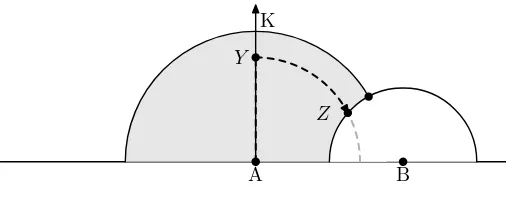
To show that each center has connected territory, consider the following. Let Abe a center, necessarily located at the boundary ofH, and letDA=ψ−1
H (A) be it’s territory. Consider the ray AA′, perpendicular to R. If some point xonAA′ doesn’t belong to DA, that’s because
the center got sated before reachingx, so no further point onAA′ belongs toDA. Thus the
A K
B
Y
Z
Figure 2: Every point ofDA can be reached fromA
Now consider an arc of a circle centered inAand intersectingAKin some pointY, and follow this arc to the right (or left) from Y. Once we meet a pointZ /∈DA, there must be a center
B such thatBZ ≤AZ, so no further points on the arc belong toDA. Thus every point ofDA can be reached fromA, andDA is connected.
Now apply the inverse mapf−1
toψH. i.e. letψ=f−1
ψHf. Clearly,ψis an allocation ofR2 to X with appetite α, and from the previous lemma it doesn’t depend on the choice off.
Lemma 2.2. The allocation ψ is translation-invariant, i.e. ifτ :R2
→R2
is a translation, andψ′ it the allocation orR2
toτ X constructed using the above procedure, thenψ′=τ−1
ψτ. Proof. LetX′=τ X. Clearly, the minimal spanning forest is translation-invariant, i.e. T′:= M SF(X′) =τ·M SF(X). Nowf′ =f τ−1
is a conformal function that maps R2
\T′ to H,
Lemma 2.3. Under the allocation ψevery center is sated a.s.
Proof. First, it follows from the Gale-Shapley algorithm (see Appendix II below), that no stable allocation may have both unclaimed sites and unsated centers. By ergodicity, the exis-tence of unclaimed sites is a 0/1 event; thus we may assume thatψH, and therefore ψ, have no unclaimed sites.
Now Lemma 16 in [1] states that for any translation-invariant allocationψ and anyr >0
P{|ψ(0)|< r}=E∗Lψ−1
(0)∩B(0, r),
where E∗ denotes the expectation with respect to the Poisson process conditioned to have a
center in 0. Takingr→ ∞yields
P{0 is claimed}=E∗Lψ−1 (0).
But we assumed the probability on the left to be equal to 1, andLψ−1
(0)≤1 by construction (a center cannot allocate more than it’s appetite), thus the lemma follows.
We summarize the above lemmas in the following
3
Further questions
Geometry of territories. Is it true that the every territory ψ−1
(ξ) is bounded a.s.? The territories ofψare connected, but, a priori, may be not simply connected (more exactly, their closures may not be simply connected). Can the construction ofψbe modified to assure this? Point process on R. What can be told about the image ofX under the Riemann map, as a
point process onR? Simulations suggest that this process should have extremely high variation of point density; even for small polygons of 30-40 points, the distances between the images of consecutive points may vary from≈1 to≈10−16
.
Fixing the Riemann map. The Riemann map f is unique up to a conformal automorphism ofH, z→az+b. Is it possible to pick (deterministically) one particular mapping from this class? If omitting the translation-invariance, one obvious way to do this is to pick a mapping
f that sends 0 toi. If doing this in translation-invariant manner, there is obviously no way to fix the shift b (since this would imply the deterministic translation-invariant choice of single point from the Poisson process). But does there exist a way to pick the scale, i.e. fix the parametera?
References
[1] Christopher Hoffman, Alexander E. Holroyd, and Yuval Peres. A stable marriage of Poisson and Lebesgue. Annals of Probability, 34:1241, 2006, math.PR/0505668. MR2257646 [2] Kenneth S. Alexander. Percolation and minimal spanning forests in infinite graphs.Annals
of Probability, 23:87–104, 1995. MR1330762
[3] Sourav Chatterjee, Ron Peled, Yuval Peres, and Dan Romik. Gravitational allocation to Poisson points, 2006, math.PR/0611886.
[4] Russell Lyons, Yuval Peres, and Oded Schramm. Minimal spanning forests. Annals of Probability, 34:1665, math.PR/0412263. MR2271476
Appendix I: An obligatory picture
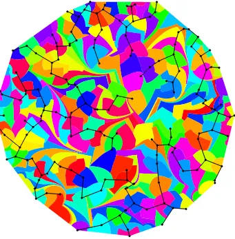
Figure 3: An approximation of allocation for 164 points in the unit circle
On the above picture we took 164 uniformly distributed points inside the unit circle, and mapped each component Kj of their convex hull minus their MST to a region ofH, so that all the internal edges are mapped toR. Then for each component we allocated it’s whole area
to the bounding corners, choosing the appetites proportional to the angular measure.
The mapping was approximated with a version of thegeodesic algorithm, adapted for domains with non-Jordan boundary (or more exactly, for domains with boundary consisting of a Jordan curve plus a number of internal trees); for discussion of numeric algorithms for quasi-conformal mappings see e.g. [5] and references therein.
Appendix II: site-optimal Gale-Shapley algorithm
(The description of the G-S algorithm below is taken from [1] except for the last step, when we have to be more careful with the definition of ψ onW in order to assure the connectedness of the territories.)
LetW be the set of all sites, equidistant from one or more centers. Since the set of centers is countable,W has Lebesgue measure null.
We construct ψ on R2
\W by means of a sequence of stages, where stage n, n = 1,2,3, . . .
consists of two steps:
a) Each sitex /∈ W applies to the closest center, which has not rejected xat any earlier stage.
b) For each centerξ, letAn(ξ) be the set of sites which applied toξon step a of stage n, and define therejection radiusas
rn(ξ) = inf{r:L(An(ξ)∩B(ξ, r))≥α},
where the infimum over the empty set is taken to be ∞. Thenξ shortlists all sites in
An(ξ)∩B(ξ, rn(ξ)), andrejectsall sites inAn(ξ)\B(ξ, rn(ξ)).
Now either x is rejected by every center (in order of increasing distance from x), or x is shortlisted byξfor some centerξat some stagen. In the former case we putψ(x) =∞(sox
is unclaimed), in the latter case we putψ(x) =ξ.
Finally, for x ∈ W put ψ(x) = ξ, if ξ is the only center such that x ∈ ∂ψ−1
(ξ), and put