El e c t ro n ic
Jo ur n
a l o
f P
r o b
a b i l i t y
Vol. 13 (2008), Paper no. 3, pages 26–78. Journal URL
http://www.math.washington.edu/~ejpecp/
The cutoff phenomenon for ergodic Markov processes
Guan-Yu Chen∗
Department of Mathematics National Chiao Tung University
Hsinchu 300, Taiwan Email:[email protected]
Laurent Saloff-Coste†
Malott Hall, Department of Mathematics Cornell University
Ithaca, NY 14853-4201 Email:[email protected]
Abstract
We consider the cutoff phenomenon in the context of families of ergodic Markov transition functions. This includes classical examples such as families of ergodic finite Markov chains and Brownian motion on families of compact Riemannian manifolds. We give criteria for the existence of a cutoff when convergence is measured inLp-norm, 1< p <
∞. This allows us to prove the existence of a cutoff in cases where the cutoff time is not explicitly known. In the reversible case, for 1< p≤ ∞, we show that a necessary and sufficient condition for the existence of a max-Lp cutoff is that the product of the spectral gap by the max-Lp mixing time tends to infinity. This type of condition was suggested by Yuval Peres. Illustrative examples are discussed.
Key words: Cutoff phenomenon, ergodic Markov semigroups. AMS 2000 Subject Classification: Primary 60J05,60J25.
Submitted to EJP on May 29, 2007, final version accepted January 8, 2008.
∗
First author partially supported by NSF grant DMS 0306194 and NCTS, Taiwan
†
1
Introduction
Let K be an irreducible aperiodic Markov kernel with invariant probability π on a finite state space Ω. LetKxl =Kl(x,·) denote the iterated kernel. Then
lim
l→∞K l x =π
and this convergence can be studied in various ways. Set kl
x =Kxl/π (this is the density of the
For p= 1, this is (twice) the total variation distance betweenKl
x and π. Forp= 2, this is the
so-called chi-square distance.
In this context, the idea of cutoff phenomenon was introduced by D. Aldous and P. Diaconis in [1; 2; 3] to capture the fact that some ergodic Markov chains converge abruptly to their invariant distributions. In these seminal works convergence was usually measured in total variation. See also [9; 21; 29] where many examples are described. The first example where a cutoff in total variation was proved (although the term cutoff was actually introduced in later works) is the random transposition Markov chain on the symmetric group studied by Diaconis and Shahshahani in [13]. One of the most precise and interesting cutoff result was proved by D. Aldous [1] and improved by D. Bayer and P. Diaconis [4]. It concerns repeated riffle shuffles. We quote here Bayer and Diaconis version for illustration purpose.
Theorem 1.1 ([4]). Let Pnl denote the distribution of a deck of n cards after l riffle shuffles (starting from the deck in order). Letunbe the uniform distribution and set l= (3/2) log2n +c.
As this example illustrates, the notion of cutoff is really meaningful only when applied to a family of Markov chains (here, the family is indexed by the number of cards). Precise definitions are given below in a more general context.
Proving results in the spirit of the theorem above turns out to be quite difficult because it often requires a very detailed analysis of the underlying family of Markov chains. At the same time, it is believed that the cutoff phenomenon is widely spread and rather typical among fast mixing Markov chains. Hence a basic natural question is whether or not it is possible to prove that a family of ergodic Markov chains has a cutoff without studying the problem in excruciating detail and, in particular, without having to determine the cutoff time. In this spirit, Yuval Peres proposed a simple criterion involving only the notion of spectral gap and mixing time.
(and, to some extent,Dp with 1< p≤ ∞). Unfortunately, for the very natural total variation
distance (i.e., the casep= 1), the question is more subtle and no good general answer is known (other measuring tools such as relative entropy and separation will also be briefly mentioned later).
Although the cutoff phenomenon has mostly been discussed in the literature for finite Markov chains, it makes perfect sense in the much more general context of ergodic Markov semigroups. For instance, on a compact Riemannian manifold, letµtbe the distribution of Brownian motion
at time t, started at some given fixed point x at time 0. In this case, the density of µt with
respect to the underlying normalized Riemannian measure is the heat kernel h(t, x,·). Now, given a sequence of Riemannian Manifolds Mn, we can ask whether or not the convergence of
Brownian motion to its equilibrium presents a cutoff. Anticipating the definitions given later in this paper, we state the following series of results which illustrates well the spirit of this work.
Theorem 1.2. Referring to the convergence of Brownian motion to its stationary measure on a family (Mn) of compact Riemannian manifolds, we have:
1. If all manifolds in the family have the same dimension and non-negative Ricci curvature, then there is no max-Lp cutoff, for anyp, 1≤p≤ ∞.
2. If for each n, Mn = Sn is the (unit) sphere in Rn+1 then, for each p ∈ [1,∞) (resp.
p=∞), there is a max-Lp cutoff at time tn= log2nn (resp. tn= lognn) with strongly optimal window1/n.
3. If for each n, Mn = SO(n) (the special orthogonal group of n by n matrices, equipped with its canonical Killing metric) then, for each p ∈ (1,∞], there is a max-Lp cutoff at time tn with window 1. The exact time tn is not known but, for any η ∈ (0,1), tn is asymptotically between(1−η) lognand2(1+η) lognifp∈(1,∞)and between2(1−η) logn
and 4(1 +η) logn ifp=∞.
The last case in this theorem is the most interesting to us here as it illustrates the main result of this paper which provides a way of asserting that a cutoff exists even though one is not able to determine the cutoff time. Note that p= 1 (i.e., total variation) is excluded in (3) above. It is believed that there is a cutoff in total variation in (3) but no proof is known at this writing. Returning to the setting of finite Markov chains, it was mentioned above that the random transposition random walk on the symmetric groupSn was the first example for which a cutoff
was proved. The original result of [13] shows (essentially) that random transposition has a cutoff both in total variation and in L2 (i.e., chi-square distance) at time 12nlogn. It may be surprising then that for great many other random walks on Sn (e.g., adjacent transpositions,
random insertions, random reversals, ...), cutoffs and cutoff times are still largely a mystery. The main result of this paper sheds some light on these problems by showing that, even if one is not able to determine the cutoff times, all these examples presentL2-cutoffs.
Theorem 1.3. For each n, consider an irreducible aperiodic random walk on the symmetric groupSn driven by a symmetric probability measurevn. Letβn be the second largest eigenvalue, in absolute value. Assume that infnβn>0 and set
σn=
X
x∈Sn
If |σn|< βn or |σn|=βn butx7→sgn(x) is not the only eigenfunction associated to ±βn, then, for any fixed p∈(1,∞], this family of random walks onSn has a max-Lp cutoff
To see how this applies to the adjacent transposition random walk, i.e.,vnis uniform on{Id,(i, i+
1),1≤i≤n−1}, recall that 1−βn is of order 1/n3 in this case whereas one easily computes
thatσn=−1 + 2/n. See [29] for details and further references to the literature.
The crucial property of the symmetric group Sn used in the theorem above is that most
irre-ducible representations have high multiplicity. This is true for many family of groups (most simple groups, either in the finite group sense or in the Lie group sense). The following theo-rem is stated for special orthogonal groups but it holds also for any of the classical families of compact Lie groups. Recall that a probability measurev on a compact group G is symmetric ifv(A) = v(A−1). Convolution by a symmetric measure is a self-adjoint operator on L2(G). If there existslsuch that thel-th convolution powerv(l)is absolutely continuous with a continuous density then this operator is compact.
Theorem 1.4. For eachn, consider a symmetric probability measurevnon the special orthogonal groupSO(n) and assume that there exists ln such thatvn(ln) is absolutely continuous with respect to Haar measure and admits a continuous density. Let βn be the second largest eigenvalue, in absolute value, of the operator of convolution by vn. Assume that infnβn > 0. Then, for any fixed p∈(1,∞], this family of random walks on SO(n) has a max-Lp cutoff.
Among the many examples to which this theorem applies, one can consider the family of random planar rotations studied in [24] which are modelled by first picking up a random plane and then making a θrotation. In the case θ=π, [24] proves a cutoff (both in total variation and in L2) at time (1/4)nlogn. Other examples are in [22; 23].
Another simple but noteworthy application of our results concerns expander graphs. For sim-plicity, for any fixed k, say that a family (Vn, En) of finite non-oriented k-regular graphs is a
family of expanders if (a) the cardinality|Vn|of the vertex set Vn tends to infinity with n, (b)
there exists ǫ > 0 such that, for any n and any set A ⊂ Vn of cardinality at most |Vn|/2, the
number of edges between A and its complement is at least ǫ|A|. Recall that the lazy simple random walk on a graph is the Markov chain which either stays put or jumps to a neighbor chosen uniformly at random, each with probability 1/2.
Theorem 1.5. Let (Vn, En)be a family of k-regular expander graphs. Then, for anyp∈(1,∞], the associated family of lazy simple random walks presents a max-Lp cutoff as well as an Lp
cutoff from any fixed sequence of starting points.
We close this introduction with remarks regarding practical implementations of Monte Carlo Markov Chain techniques. In idealized MCMC practice, an ergodic Markov chain is run in order to sample from a probability distribution of interest. In such situation, one can often identify parameters that describe the complexity of the task (in card shuffling examples, the number of cards). For simplicity, denote bynthe complexity parameter. Now, in order to obtain a “good” sample, one needs to determine a “sufficiently large” running timeTn to be used in the sampling
of Markov chains underlying the sampling algorithm (indexed by the complexity parameter
n) presents a cutoff at time tn then the optimal sufficient running time Tn is asymptotically
equivalent totn. If there is a cutoff at timetn with window size bn (by definition, this implies
that bn/tn tends to 0), then one gets the more precise result that the optimal running time Tn
should satisfy |Tn−tn|= O(bn) as n tends to infinity. The crucial point here is that, if there
is a cutoff, these relations hold for any desired fixed admissible error size whereas, if there is no cutoff, the optimal sufficient running timeTndepends greatly of the desired admissible error
size.
Now, in the discussion above, it is understood that errors are measured in some fixed acceptable way. The chi-square distance at the center of the present work is a very strong measure of convergence, possibly stronger than desirable in many applications. Still, what we show is that in any reversible MCMC algorithm, assuming that errors are measured in chi-square distance, if any sufficient running time is much longer than the relaxation time (i.e., the inverse of the spectral gap) then there is a cutoff phenomenon. This means that for any such algorithm, there is an asymptotically well defined notion of optimal sufficient running time as discussed above (with window size equal to the relaxation time). This work says nothing however about how to find this optimal sufficient running time.
Description of the paper
In Section 2, we introduce the notion of cutoff and its variants in a very general context. We also discuss the issue of optimality of the window of a cutoff. This section contains technical results whose proofs are in the appendix.
In Section 3, we introduce the general setting of Markov transition functions and discuss Lp
cutoffs from a fixed starting distribution.
Section 4 treats max-Lp cutoffs under the hypothesis that the underlying Markov operators are normal operators. In this case, a workable necessary and sufficient condition is obtained for the existence of a max-Lp cutoff when 1< p <∞.
In Section 5, we consider the reversible case and the normal transitive case (existence of a transitive group action). In those cases, we show that the existence of a max-Lp cutoff is
independent ofp∈(1,∞). In the reversible case,p= +∞ is included.
Finally, in Section 6, we briefly describe examples proposed by David Aldous and by Igor Pak that show that the criterion obtained in this paper in the case p ∈ (1,∞) does not work for
p= 1 (i.e., in total variation).
2
Terminology
This section introduces some terminology concerning the notion of cutoff. We give the basic definitions and establish some relations between them in a context that emphasizes the fact that no underlying probability structure is needed.
2.1 Cutoffs
Definition 2.1. Forn≥1, letDn⊂[0,∞) be an unbounded set containing 0. Letfn :Dn→
[0,∞] be a non-increasing function vanishing at infinity. Assume that
M = lim sup
n→∞ fn(0)>0. (2.1)
Then the family F ={fn:n= 1,2, ...} is said to present
(c1) a precutoff if there exist a sequence of positive numbers tn and b > a >0 such that
lim
n→∞t>btsupn
fn(t) = 0, lim inf n→∞ t<atinfn
fn(t)>0.
(c2) a cutoff if there exists a sequence of positive numbers tnsuch that
lim
n→∞t>(1+supǫ)tnfn(t) = 0, nlim→∞t<(1inf−ǫ)tn
fn(t) =M,
for allǫ∈(0,1).
(c3) a (tn, bn) cutoff if tn>0,bn≥0,bn=o(tn) and
lim
c→∞F(c) = 0, c→−∞lim F(c) =M,
where, for c∈R,
F(c) = lim sup
n→∞ t>tsupn+cbn
fn(t), F(c) = lim inf
n→∞ t<tinfn+cbn
fn(t). (2.2)
Regarding (c2) and (c3), we sometimes refer informally to tn as a cutoff sequence and bn as a
window sequence.
Remark 2.1. In (c3), sincefn might not be defined attn+cbn, we have to take the supremum
and the infimum in (2.2). However, ifDn= [0,∞) andbn>0, then a (tn, bn) cutoff is equivalent
to ask limc→∞G(c) = 0 and limc→−∞G(c) =M, where forc∈R,
G(c) = lim sup
n→∞ fn(tn+cbn), G(c) = lim infn→∞ fn(tn+cbn).
Remark 2.2. To understand and picture what a cutoff entails, letF be a family as in Definition 2.1 withDn≡[0,∞) and let (tn)∞1 be a sequence of positive numbers. Setgn(t) =fn(tnt) for
t >0 and n≥1. Then F has a precutoff if and only if there exist b > a > 0 and tn> 0 such
that
lim
n→∞gn(b) = 0, lim infn→∞ gn(a)>0.
Similarly, F has a cutoff with cutoff sequence tn if and only if
lim
n→∞gn(t) =
(
0 fort >1
M for 0< t <1
Remark 2.3. Obviously, (c3)⇒(c2)⇒(c1). In (c3), if, forn≥1,Dn= [0,∞) andfnis continuous,
then the existence of a (tn, bn) cutoff implies thatbn>0 for nlarge enough.
Remark 2.4. It is worth noting that another version of cutoff, called a weak cutoff, is introduced by Saloff-Coste in [28]. By definition, a family F as above is said to present a weak cutoff if there exists a sequence of positive numberstn such that
∀ǫ >0, lim
n→∞t>(1+supǫ)tnfn(t) = 0, lim infn→∞ t<tinfn
fn(t)>0.
It is easy to see that the weak cutoff is stronger than the precutoff but weaker than the cutoff. The weak cutoff requires a positive lower bound on the left limit offnattn whereas the cutoffs
in (c1)-(c3) require no information on the values offnin a small neighborhood oftn. This makes
it harder to find a cutoff sequence for a weak cutoff and differentiates the weak cutoff from the notions considered above.
The following examples illustrate Definition 2.1. Observe that the functions fn below are all
sums of exponential functions. Such functions appear naturally when the chi-square distance is used in the context of ergodic Markov processes.
Example 2.1. Fixα >0. Forn≥1, letfn be an extended function on [0,∞) defined by fn(t) =
P
k≥1e−tk α/n
. Note thatfn(0) =∞ forn≥1. This implies M = lim supn→∞fn(0) =∞. We
shall prove that F has no precutoff. To this end, observe that sincekα ≥1 +αlogk,k≥1, we have
e−t/n≤fn(t)≤e−t/n ∞
X
k=1
k−αt/n, ∀t≥0, n≥1. (2.3)
Let tn and b be positive numbers such that fn(btn) → 0. The first inequality above implies
tn/n → ∞. The second inequality gives fn(atn) = O(e−atn/n) for all a > 0. Hence, we must
have fn(atn)→0 for all a >0. This rules out any precutoff.
Example 2.2. LetF ={fn:n ≥1}, where fn(t) =Pk≥1nke−tk/n for t≥0 and n≥1. Then
fn(t) =∞ fort∈[0, nlogn] andfn(t) =ne−t/n/(1−ne−t/n) fort > nlogn. This implies that
M =∞. Settingtn=nlogn andbn=n, the functionsF and F defined in (2.2) are given by
F(c) =F(c) = (
e−c
1−e−c ifc >0
∞ ifc≤0 (2.4)
Hence,F has a (nlogn, n) cutoff.
Example 2.3. Let F ={fn:n≥1}, wherefn(t) = (1 +e−t/n)n−1 fort≥0,n≥1. Obviously,
M =∞. In this case, setting tn=nlognand bn=nyields
F(c) =F(c) =ee−c−1, ∀c∈R. (2.5)
This proves thatF has the (nlogn, n) cutoff.
2.2 Window optimality
It is clear that the quantitybn in (c3) reflects the sharpness of a cutoff and may depend on the
Definition 2.2. LetF andM be as in Definition 2.1. Assume thatF presents a (tn, bn) cutoff.
Then, the cutoff is
(w1) weakly optimal if, for any (tn, dn) cutoff for F, one hasbn=O(dn).
(w2) optimal if, for any (sn, dn) cutoff forF, we havebn =O(dn). In this case, bn is called an
optimal window for the cutoff.
(w3) strongly optimal if, for allc >0,
0<lim inf
n→∞ t>tsupn+cbn
fn(t)≤lim sup
n→∞ t<tinfn−cbn
fn(t)< M.
Remark 2.5. Obviously, (w3)⇒(w2)⇒(w1). If F has a strongly optimal (tn, bn) cutoff, then
bn > 0 for n large enough. If Dn is equal to N for all n ≥1, then a strongly optimal (tn, bn)
cutoff for F implies lim inf
n→∞ bn>0.
Remark 2.6. Let F be a family of extended functions defined onN. If F has a (tn, bn) cutoff withbn→0, it makes no sense to discuss the optimality of the cutoff and the window. Instead,
it is worthwhile to determine the limsup and liminf of the sequences
fn([tn] +k) fork=−1,0,1.
See [7] for various examples.
Remark 2.7. Let F be a family of extended functions presenting a strongly optimal (tn, bn)
cutoff. IfT = [0,∞) then there existN >0 and 0< c1 < c2 < M such thatc1 ≤fn(tn)≤c2 for alln > N. In the discrete time case whereT =N, we have insteadc1 ≤fn(⌈tn⌉)≤fn(⌊tn⌋)≤c2 for all n > N.
The following lemma gives an equivalent definition for (w3) using the functions in (2.2).
Lemma 2.1. Let F be a family as in Definition 2.1 with Dn=Nfor all n≥1 or Dn= [0,∞) for all n ≥1. Assume (2.1) holds. Then a family presents a strongly optimal (tn, bn) cutoff if and only if the functions, F and F, defined in (2.2) with respect to tn, bn satisfy F(−c) < M and F(c)>0 for all c >0.
Proof. See the appendix.
Our next proposition gives conditions that are almost equivalent to the various optimality condi-tions introduced in Definition 2.2. These are useful in investigating the optimality of a window.
Proposition 2.2. Let F = {fn, n = 1,2, ...} be a family of non-increasing functions fn :
[0,∞)→ [0,∞] vanishing at infinity. SetM = lim supnfn(0). Assume that M >0 and that F has a(tn, bn) cutoff withbn>0. For c∈R, let
G(c) = lim sup
n→∞
fn(tn+cbn), G(c) = lim inf
n→∞ fn(tn+cbn). (2.6)
(ii) If there existc2 > c1 such that0< G(c2)≤G(c1)< M, then the(tn, bn) cutoff is optimal. Conversely, if the(tn, bn) cutoff is optimal, then there arec2 > c1 such thatG(c2)>0and
G(c1)< M.
(iii) The (tn, bn) cutoff is strongly optimal if and only if 0< G(c)≤G(c)< M for all c∈R. In particular, if(tn, bn) is an optimal cutoff and there exists c∈Rsuch that G(c) =M or
G(c) = 0, then there is no strongly optimal cutoff for F.
Remark 2.8. Proposition 2.2 also holds if one replacesG, G withF , F defined at (2.2).
Remark 2.9. Consider the case whenfnhas domain N. Assume that lim infnbn>0 and replace
G, G in Proposition 2.2 with F , F defined at (2.2). Then (iii) remains true whereas the first parts of (i),(ii) still hold if, respectively,
lim inf
n→∞ bn>2/c, lim infn→∞ bn>4/(c2−c1).
The second parts of (i),(ii) hold if we assume lim supnbn=∞.
Example 2.4 (Continuation of Example 2.2). Let F be the family in Example 2.2. By (2.4),
F has a (tn, n) cutoff with tn = nlogn. Suppose F has a (tn, cn) cutoff. By definition, since
fn(tn+n) = 1/(e−1), we may choose C >0, N >0 such that
fn(tn+Ccn)< fn(tn+n), ∀n≥N.
This impliesn=O(cn) and, hence, the (nlogn, n) cutoff is weakly optimal. We will prove later
in Example 2.6 that such a cutoff is optimal but that no strongly optimal cutoff exists.
Example2.5 (Continuation of Example 2.3). For the familyF in Example 2.3, (2.5) implies that the (nlogn, n) cutoff is strongly optimal.
2.3 Mixing time
The cutoff phenomenon in Definition 2.1 is closely related to the way each function inF tends to 0. To make this precise, consider the following definition.
Definition 2.3. Letf be an extended real-valued non-negative function defined onD⊂[0,∞). Forǫ >0, set
T(f, ǫ) = inf{t∈D:f(t)≤ǫ}
if the right hand side above is non-empty and letT(f, ǫ) =∞ otherwise.
In the context of ergodic Markov processes,T(fn, ǫ) appears as the mixing time. This explains
the title of this subsection.
Proposition 2.3. Let F = {fn : [0,∞) → [0,∞]|n = 1,2, ...} be a family of non-increasing functions vanishing at infinity. Assume that (2.1)holds. Then:
(i) F has a precutoff if and only if there exist constants C ≥ 1 and δ > 0 such that, for all 0< η < δ,
lim sup
n→∞
T(fn, η)
T(fn, δ) ≤
(ii) F has a cutoff if and only if (2.7)holds for all 0< η < δ < M with C= 1.
(iii) For n≥1, let tn>0, bn≥0 be such that bn=o(tn). ThenF has a(tn, bn) cutoff if and only if, for all δ∈(0, M),
|tn−T(fn, δ)|=Oδ(bn). (2.8)
Proof. The proof is similar to that of the next proposition.
Remark 2.10. If (2.7) holds for 0 < η < δ < M with C = 1, then T(fn, η) ∼ T(fn, δ) for all
0< η < δ < M, where, for two sequences of positive numbers (tn) and (sn),tn∼sn means that
tn/sn→1 as n→ ∞.
Proposition 2.4. LetF ={fn:N→[0,∞]|n= 1,2, ...}be a family of non-increasing functions vanishing at infinity. Let M be the limit defined in (2.1). Assume that there exists δ0 >0 such that
lim
n→∞T(fn, δ0) =∞. (2.9)
Then (i) and (ii) in Proposition 2.3 hold. Furthermore, ifbn satisfies
lim inf
n→∞ bn>0, (2.10)
then (iii) in Proposition 2.3 holds.
Proof. See the appendix.
Remark 2.11. A similar equivalent condition for a weak cutoff is established in [6]. In detail, referring to the setting of Proposition 2.3 and 2.4, a familyF ={fn :n= 1,2, ...} has a weak
cutoff if and only if there exists a positive constant δ > 0 such that (2.7) holds for 0 < η < δ
withC = 1.
Remark 2.12. More generally, if F is the family introduced in Definition 2.1, then Proposition 2.3 holds when Dn is dense in [0,∞) for all n ≥ 1. Proposition 2.4 holds when [0,∞) =
S
x∈Dn(x−r, x+r) for all n≥1, where r is a fixed positive constant. This fact is also true for the equivalence of the weak cutoff in Remark 2.11.
A natural question concerning cutoff sequences arises. Suppose a family F has a cutoff with cutoff sequence (sn)∞1 and a cutoff with cutoff sequence (tn)∞1 . What is the relation between
sn and tn? The following corollary which follows immediately from Propositions 2.3 and 2.4
answers this question.
Corollary 2.5. Let F be a family as in Proposition 2.3 satisfying (2.1)or as in Proposition 2.4 satisfying (2.9).
(i) If F has a cutoff, then the cutoff sequence can be taken to be (T(fn, δ))∞1 for any0< δ <
M.
(ii) F has a cutoff with cutoff sequence (tn)∞1 if and only if tn∼T(fn, δ) for all0< δ < M.
In the following, ifF is the family in Proposition 2.4, we assume further that the sequence(bn)∞1 satisfies (2.10).
(iv) If F has a (tn, bn) cutoff, then F has a(T(fn, δ), bn) cutoff for any0< δ < M.
(v) Assume that F has a (tn, bn) cutoff. Let sn >0 and dn ≥0 be such that dn=o(sn) and
bn=O(dn). Then F has a (sn, dn) cutoff if and only if |tn−sn|=O(dn).
The next corollaries also follow immediately from Propositions 2.3 and 2.4. They address the optimality of a window.
Corollary 2.6. Let F be a family in Proposition 2.3 satisfying (2.1). Assume that F has a cutoff. Then the following are equivalent.
(i) bn is an optimal window.
(ii) F has an optimal (T(fn, δ), bn) cutoff for some 0< δ < M.
(iii) F has a weakly optimal (T(fn, δ), bn) cutoff for some 0< δ < M.
Proof. (ii)⇒(iii) is obvious. For (i)⇒(ii), assume thatF has a (tn, bn) cutoff. Then, by
Propo-sition 2.3,F has a (T(fn, δ), bn) cutoff for all δ ∈ (0, M). The optimality is obvious from that
of the (tn, bn) cutoff. For (iii)⇒(i), assume that F has a (sn, cn) cutoff. By Proposition 2.3, F
has a (T(fn, δ), cn) cutoff. Consequently, the weak optimality implies thatbn=O(cn).
Remark 2.13. In the case whereF consists of functions defined on [0,∞), there is no difference between a weakly optimal cutoff and an optimal cutoff if the cutoff sequence is selected to be (T(fn, δ))∞1 for some 0< δ < M.
Corollary 2.7. Let F be as in Proposition 2.4 satisfying (2.9) and (bn)∞1 be such that lim inf
n→∞ bn>0. Assume that F has a cutoff. Then the following are equivalent.
(i) bn is an optimal window.
(ii) For some δ∈(0, M), the family F has both weakly optimal (T(fn, δ), bn) and (T(fn, δ)−
1, bn) cutoffs.
Proof. See the appendix.
Example 2.6 (Continuation of Example 2.2). In Example 2.2, the family F has been proved to have a (nlogn, n) cutoff and the functions F , F are computed out in (2.4). We noticed in Example 2.4 that this is weakly optimal. By Lemma 2.8, we may conclude from (2.4) thatnis an optimal window and also that no strongly optimal cutoff exists. Indeed, the forms of F , F
show that the optimal “right window” is of ordernbut the optimal “left window” is 0. Since our definition for an optimal cutoff is symmetric, the optimal window should be the larger one and no strongly optimal window can exist. The following lemma generalizes this observation.
(i) Assume that either F >0 or F < M. Then the (tn, bn) cutoff is optimal.
(ii) Assume that either F > 0 with F(c) =M for some c∈ R or F < M with F(c) = 0 for some c∈R. Then there is no strongly optimal cutoff for F.
The above is true for a family as in Proposition 2.4 if we assume further lim inf
n→∞ bn>0.
Proof. See the appendix.
The following proposition compares the window of a cutoff between two families. This is useful in comparing the sharpness of cutoffs when two families have the same cutoff sequence.
Proposition 2.9. LetF ={fn:n≥1}andG={gn:n≥1} be families both as in Proposition 2.3 or 2.4 and set
lim sup
n→∞ fn(0) =M1, lim supn→∞ gn(0) =M2.
Assume thatM1 >0 and M2 >0. Assume further that F has a strongly optimal (tn, bn) cutoff and that G has a(sn, cn) cutoff with|sn−tn|=O(bn). Then:
(i) If fn≤gn for all n≥1, then bn=O(cn).
(ii) If M1=M2 and, forn≥1, either fn≥gn or fn≤gn, then bn=O(cn).
Proof. See the appendix.
3
Ergodic Markov processes and semigroups
3.1 Transition functions, Markov processes
As explained in the introduction, the cutoff phenomenon was originally introduced in the con-text of finite Markov chains. However, it makes sense in the much larger concon-text of ergodic Markov processes. In what follows, we let time be either continuous t ∈ [0,∞) or discrete
t∈ {0,1,2, . . . ,∞}=N.
A Markov transition function on a space Ω equipped with aσ-algebraB, is a family of probability measuresp(t, x,·) indexed by t∈T (T = [0,∞) or N) and x ∈Ω such thatp(0, x,Ω\ {x}) = 0 and, for eacht∈T and A∈ B,p(t, x, A) isB-measurable and satisfies
p(t+s, x, A) = Z
Ω
p(s, y, A)p(t, x, dy).
A Markov process X = (Xt, t ∈T) with filtrationFt =σ(Xs :s≤t)⊂ B hasp(t, x,·), t ∈T,
x∈Ω, as transition function provided
E(f◦Xs|Ft) =
Z
Ω
for all 0< t < s <∞and all bounded measurablef. The measureµ0(A) =P(X0 ∈A) is called the initial distribution of the processX. All finite dimensional marginals ofX can be expressed in terms ofµ0 and the transition function. In particular,
µt(A) =P(Xt∈A) =
Z
p(t, x, A)µ0(dx).
Given a Markov transition functionp(t, x,·),t∈T, x∈Ω, for any bounded measurable function
f, set
Ptf(x) =
Z
f(y)p(t, x, dy).
For any measureν on (Ω,B) with finite total mass, set
νPt(A) =
Z
p(t, x, A)ν(dx).
We say that a probability measureπ is invariant ifπPt=π for allt∈T. In this general setting,
invariant measures are not necessarily unique.
Example 3.1 (Finite Markov chains). A (time homogeneous) Markov chain on finite state space Ω is often described by its Markov kernelK(x, y) which gives the probability of moving fromx
toy. The associated discrete time transition functionpd(t,·,·) is defined inductively for t∈N,
x, y∈Ω, by pd(0, x, y) =δ
x(y) and
pd(1, x, y) =K(x, y), pd(t, x, y) =X
z∈Ω
pd(t−1, x, z)pd(1, z, y). (3.1)
The associated continuous time transition functionpc(t,·,·) is defined fort≥0 and x, y∈Ω by
pc(t, x, y) =e−t
∞
X
j=0
tj j!p
d(j, x, y). (3.2)
One says that K is irreducible if, for any x, y∈ Ω, there exists l∈ N such that pd(l, x, y)>0. For irreducibleK, there exists a unique invariant probabilityπ such thatπK =π and pc(t, x,·)
tends to π asttends to infinity.
3.2 Measure of ergodicity
Our interest here is in the case where some sort of ergodicity holds in the sense that, for some initial measure µ0, µ0Pt converges (in some sense) to a probability measure. By a simple
argument, this limit must be an invariant probability measure. In order to state our main results, we need the following definition.
Definition 3.1. Let p(t, x,·), t ∈ T, x ∈ Ω, be a Markov transition function with invariant measure π. We call spectral gap (of this Markov transition function) and denote by λ the largest c≥0 such that, for allt∈T and allf ∈L2(Ω, π),
Remark 3.1. IfT = [0,∞) and Ptf tends to f inL2(Ω, π) ast tends to 0 (i.e.,Pt is a strongly
continuous semigroup of contractions on L2(Ω, π)) then λ can be computed in term of the infinitesimal generatorA of Pt=etA. Namely,
λ= inf{h−Af, fi:f ∈Dom(A), real valued, π(f) = 0, kfk2 = 1}.
Note that A is not self-adjoint in general and thus λ is not always in the spectrum ofA (it is in the spectrum of the self-adjoint operator 12(A+A∗)). If A is self-adjoint then λ measures the gap between the smallest element of the spectrum of −A (which is the eigenvalue 0 with associated eigenspace the space of constant functions) and the rest of the spectrum of−Awhich lies on the positive real axis.
Remark 3.2. IfT =Nthenλis simply defined by
λ=−log¡kP1−πkL2(Ω,π)→L2(Ω,π)
¢
.
In other words,e−λ is the second largest singular value of the operatorP1 onL2(Ω, π).
Remark 3.3. If λ > 0 then limt→∞p(t, x, A) =π(A) for π almost all x. Indeed (assuming for
simplicity thatT =N), for any bounded measurable function f, we have
π(X
n
|Pnf −π(f)|2) =
X
n
k(Pn−π)(f)k2L2(Ω,π) ≤
à X
n
e−2λn
!
kfk2∞.
HencePnf(x) converges toπ(f),π almost surely.
Remark 3.4. As kPt−πkL1(Ω,π)→L1(Ω,π) and kPt−πkL∞(Ω,π)→L∞(Ω,π) are bounded by 2, the Riesz-Thorin interpolation theorem yields
kPt−πkLp(Ω,π)→Lp(Ω,π) ≤2|1−2/p|e−tλ(1−|1−2/p|). (3.4)
We now introduce the distance functions that will be used throughout this work to measure convergence to stationarity. First, set
DTV(µ0, t) =kµ0Pt−πkTV= sup
A∈B{|
µ0Pt(A)−π(A)|}.
This is the total variation distance between probability measures.
Next, fix p ∈ [1,∞]. If t is such that the measure µ0Pt is absolutely continuous w.r.t. π with
densityh(t, µ0, y), set
Dp(µ0, t) = µZ
Ω|
h(t, µ0, y)−1|pπ(dy) ¶1/p
, (3.5)
(understood asD∞(µ0, t) =kh(t, µ0,·)−1k∞whenp=∞). Ifµ0Ptis not absolutely continuous
with respect toπ, setD1(µ0, t) = 2 and, forp >1,Dp(µ0, t) =∞. When µ0 =δx, we write
h(t, x,·) forh(t, δx,·) and Dp(x, t) forDp(δx, t).
Note thatt7→Dp(x, t) is well defined for every starting pointx.
The main results of this paper concern the functionsDp with p∈(1,∞]. For completeness, we
• Separation: use sep(µ0, t) = supy{1−h(t, µ0, y)} if the density exists, sep(µ0, t) = 1, otherwise.
• Relative entropy: use Entπ(µ0, t) = Rh(t, µ0, y) logh(t, µ0, y)π(dy) if the density exists, Entπ(µ0, t) =∞ otherwise.
• Hellinger: use Hπ(µ0, t) = 1− R p
h(t, µ0, y)π(dy) if the density exists, Hπ(µ0, t) = 1 otherwise.
Proposition 3.1. Let p(t, x,·), t ∈ T, x ∈ Ω, be a Markov transition function with invariant measure π. Then, for any 1 ≤ p ≤ ∞, and any initial measure µ0 on Ω, the function t 7→
Dp(µ0, t) from T to[0,∞]is non-increasing.
Proof. Fix 1 ≤ p ≤ ∞. Consider the operator Pt acting on bounded functions. Since π is
invariant, Jensen inequality shows thatPtextends as a contraction onLp(Ω, π). Given an initial
measureµ0, the measureµ0Ptis absolutely continuous w.r.t. πwith a density inLp(Ω, π) if and
only if there exists a constantC such that
|µ0Pt(f)| ≤Ckfkq
for allf ∈Lq(Ω, π) where 1/p+ 1/q = 1 (forp∈(1,∞], this amounts to the fact that Lp is the
dual ofLqwhereas, forp= 1, it follows from a slightly more subtle argument). Moreover, if this holds then the densityh(t, µ0,·) hasLp(Ω, π)-norm
kh(t, µ0,·)kp = sup{µ0Pt(f) :f ∈Lq(Ω, π), kfkq≤1}.
Now, observe that µt+s = µtPs with µt = µ0Pt. Also, by the invariance of π, µt+s −π =
(µt−π)Ps. Finally, for anyf ∈Lq(Ω, π),
|[µt+s−π](f)|=|[µt−π]Ps(f)|.
Hence, ifµt is absolutely continuous w.r.t.π with a densityh(t, µ0,·) inLp(Ω, π) then
|[µt+s−π](f)| ≤ kh(t, µ0,·)−1kpkPsfkq ≤ kh(t, µ0,·)−1kpkfkq.
It follows that µt+s is absolutely continuous with density h(t+s, µ0,·) in Lp(Ω, π) satisfying
Dp(µ0, t+s) =kh(t+s, µ0,·)−1kp≤ kh(t, µ0,·)−1kp =Dp(µ0, t)
as desired.
Remark 3.5. Somewhat different arguments show that total variation, separation, relative en-tropy and the Hellinger distance all lead to non-increasing functions of time.
Next, given a Markov transition function with invariant measureπ, we introduce the maximal
Lp distance over all starting points (equivalently, over all initial measures). Namely, for any fixedp∈[1,∞], set
Dp(t) =DΩ,p(t) = sup x∈Ω
Obviously, the previous proposition shows that this is a non-increasing function of time. Let us insist on the fact that the supremum is taken over all starting points. In fact, let us introduce also
e
Dπ,p(t) =π- ess sup x∈Ω
Dp(x, t). (3.7)
ObviouslyDeπ,p(t) ≤Dp(t). Note that, in general,Deπ,p(t) cannot be used to control Dp(µ0, t) unlessµ0 is absolutely continuous w.r.t.π. However, if Ω is a topological space andx7→Dp(x, t)
is continuous thenDeπ,p(t) =Dp(t).
Proposition 3.2. Let p(t, x,·), t ∈ T, x ∈ Ω, be a Markov transition function with invariant measureπ. Then, for anyp∈[1,∞], the functionst7→Dp(t)andt7→Deπ,p(t)are non-increasing and sub-multiplicative.
Proof. Assume thatt, s∈T are such thath(s, x,·) andh(t, x,·) exist and are inLp(Ω, π), for a.e.
x (otherwise there is nothing to prove). Fix such an x and observe that, for any f ∈Lq(Ω, π) with 1/p+ 1/q= 1,
p(t+s, x, f)−π(f) = [p(s, x,·)−π][Pt−π](f).
It follows that
|p(t+s, x, f)−π(f)| ≤ kh(s, x,·)−1kpk[Pt−π](f)kq
≤ kh(s, x,·)−1kpk(Pt−π)fk∞
≤ kh(s, x,·)−1kpess sup y∈Ω k
h(t, y,·)−1kpkfkq
≤ kh(s, x,·)−1kpDeπ,p(t)kfkq.
Hence
Dp(x, t+s)≤Dp(x, s)Deπ,p(t).
This is a slightly more precise result than stated in the proposition.
Remark 3.6. One of the reasons behind the sub-multiplicative property ofDp and Deπ,p is that
these quantities can be understood as operator norms. Namely,
Dp(t) = sup
½ sup
Ω {|
(Pt−π)f|}: f ∈Lq(Ω, π), kfkq= 1
¾
= kPt−πkLq(Ω,π)→B(Ω) (3.8)
where B(Ω) is the set of all bounded measurable functions on Ω equipped with the sup-norm, and
e
Dπ,p = sup
½
π- ess sup Ω {|
(Pt−π)f|}: f ∈Lq(Ω, π), kfkq= 1
¾
= kPt−πkLq(Ω,π)→L∞(Ω,π). (3.9)
3.3 Lp-cutoffs
Fixp∈[1,∞]. Consider a family of spaces Ωn indexed byn= 1,2, . . . For eachn, letpn(t, x,·),
t ∈ [0,∞), x ∈ Ωn be a transition function with invariant probability πn. Fix a subset En
of probability measures on Ωn and consider the supremum of the corresponding Lp distance
betweenµPn,t and πnoverall µ∈En, that is,
fn(t) = sup µ∈En
Dp(µ, t)
where Dp(µ, t) is defined by (3.5). One says that the sequence (pn, En) presents an Lp-cutoff
when the family of functions F ={fn, n= 1,2, . . .} presents a cutoff in the sense of Definition
2.1. Similarly, one definesLp precutoff andLp (tn, bn)-cutoff for the sequence (pn, En).
We can now state the first version of our main result.
Theorem 3.3 (Lp-cutoff, 1< p <∞). Fix p∈(1,∞). Consider a family of spaces Ω
n indexed byn= 1,2, . . . For eachn, let pn(t,·,·),t∈T,T = [0,∞)or T =N, be a transition function on
Ωn with invariant probability πn and spectral gap λn. For each n, let En be a set of probability measures onΩn and consider the supremum of the corresponding Lp distance to stationarity
fn(t) = sup µ∈En
Dp(µ, t),
where Dp(µ, t) is defined at (3.5). Assume that each fn tends to zero at infinity, fix ǫ >0 and consider the ǫ-Lp-mixing time
tn=Tp(En, ǫ) =T(fn, ǫ) = inf{t∈T :Dp(µ, t)≤ǫ,∀µ∈En}.
1. When T = [0,∞), assume that
lim
n→∞λntn=∞. (3.10)
Then the family of functionsF ={fn, n= 1, . . . ,} presents a(tn, λ−n1) cutoff.
2. When T =N, set γn= min{1, λn} and assume that
lim
n→∞γntn=∞. (3.11)
Then the family of functionsF ={fn, n= 1, . . . ,} presents a(tn, γn−1) cutoff.
If En = {µ}, we write Tp(µ, ǫ) for Tp(En, ǫ). If µ = δx, we write Tp(x, ǫ) for Tp(δx, ǫ). It is
obvious that
Tp(En, ǫ) = sup µ∈En
Tp(µ, ǫ).
In particular, ifMn is the set of probability measures on Ωn, then
Tp(Mn, ǫ) = sup x∈Ωn
Proof of Theorem 3.3. Set 1/p+ 1/q = 1. Letµn,t=µn,0Pn,t. Fix ǫ >0 and settn=Tp(En, ǫ)
and assume (as we may) thattn is finite forn large enough. Forf ∈Lq(Ωn, πn) and t=u+v,
u, v >0, we have
[µn,t−πn](f) = [µn,u−πn][Pn,v −πn](f).
Hence, using (3.4),
|[µn,t−πn](f)| ≤ Dp(µn,0, u)k[Pn,v−πn](f)kq
≤ Dp(µn,0, u)2|1−2/p|e−vλn(1−|1−2/p|)kfkq.
Taking the supremum over allf withkfkq = 1 and over allµn,0 ∈Enyields
fn(u+v)≤2|1−2/p|fn(u)e−vλn(1−|1−2/p|).
Using this with eitheru > tn, v =λn−1c, c > 0, or 0< u < tn+λ−n1c,v = −λ−n1c, c <0, (the
latterucan be taken positive fornlarge enough because, by hypothesis,tnλntends to infinity),
we obtain
F(c) = lim sup
n→∞ t>tsupn+cλ−1
n
fn(t)≤ǫ2|1−2/p|e−c(1−|1−2/p|), c >0,
and
F(c) = lim inf
n→∞ t<tn+infcλ−n1
fn(t)≥ǫ2|1−2/p|e−c(1−|1−2/p|), c <0.
This proves the desired cutoff.
Remark 3.7. In Theorem 3.3 the stated sufficient condition, i.e.,λntn→ ∞(resp. γntn→ ∞) is
also obviously necessary for a (tn, λ−n1) cutoff (resp. a (tn, γn−1) cutoff). However, it is important
to notice that these conditions are not necessary for the existence of a cutoff with cutoff timetn
and unspecified window. See Example 3.2 below.
Remark 3.8. The reason one needs to introduce γn = min{1, λn} in order to state the result
in Theorem 3.3(2) is obvious. In discrete time, it makes little sense to talk about a window of width less than 1.
Remark 3.9. The conclusion of Theorem 3.3 (in both cases (1) and (2)) is false forp= 1, even under an additional self-adjoiness assumption. Whether or not it holds true for p = ∞ is an open question in general. It does hold true for p=∞when self-adjoiness is assumed.
The following result is an immediate corollary of Theorem 3.3. It indicates one of the most common ways Theorem 3.3 is applied to prove an L2-cutoff.
Corollary 3.4 (L2-cutoff). Consider a family of spaces Ωn indexed by n = 1,2, . . . For each
n, let pn(t,·,·), t ∈ T, T = [0,∞) or T = N, be a transition function on Ωn with invariant probability πn and spectral gap λn. Assume that there exists c > 0 such that, for each n, there exist φn∈L2(Ω,, πn) and xn∈Ωn such that
|(Pn,t−πn)φn(xn)| ≥e−cλnt|φn(xn)|.
1. If T = [0,∞) and
lim
n→∞(|φn(xn)|/kφnkL2(Ωn,πn)) =∞
2. If T =N, sup
nλn<∞ and
lim
n→∞(|φn(xn)|/kφnkL2(Ωn,πn)) =∞
then the family of functionsD2(xn, t) presents a cutoff.
3.4 Some examples of cutoffs
This section illustrates Theorem 3.3 with several examples. We start with an example showing that the sufficient conditions of Theorem 3.3 are not necessary.
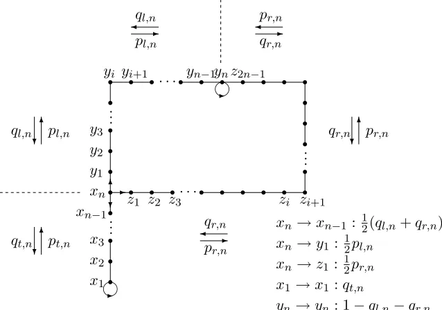
Example 3.2. Forn≥1, letKn be a Markov kernel on the finite set Ωn={0,1}n defined by
Kn(x, y) =
(
1/2 if yi+1 =xi for 1≤i≤n−1
0 otherwise (3.12)
for all x = xnxn−1· · ·x1, y = yn· · ·y1 ∈ Ωn. In other words, if we identify (Z2)n with Z2n by mapping x = xn· · ·x1 to Pixi2i−1, then Kn(x, y) > 0 if and only if y = 2x or y =
2x+ 1(mod 2n). For such a Markov kernel, letpd
n(t,·,·),pcn(t,·,·), be, respectively, the discrete
and continuous Markov transition functions defined at (3.1) and (3.2). Obviously, the unique invariant probability measure πn for both Markov transition functions is uniform on Ωn. It is
worth noting that, forn≥1, 1≤p≤ ∞andt≥0, theLp distance betweenδ
xPn,tc (resp. δxPn,td )
and πn is independent of x ∈Ωn. Hence we fix the starting point to be0 (the string of n 0s)
and set (with ∗=dorc)
fn,p∗ (t) = Ã
X
y
|(p∗n(t,0, y)/πn(y))−1|pπn(y)
!1/p
.
The following proposition shows that, for any 1≤p≤ ∞, there are cutoffs in both discrete and continuous time with tn=T(fn∗,1/2) of order nand spectral gap bounded above by 1/n. This
provides examples with a cutoff even sotnλn (ortnγn) stays bounded.
Proposition 3.5. Referring to the example and notation introduced above, let λdn and λcn be re-spectively the spectral gaps of pdn andpcn. Then λdn= 0 and λcn≤1/n.
Moreover, for any fixed p, 1≤p≤ ∞, we have:
(i) The family {fnd} has an optimal (n,1) cutoff. No strongly optimal cutoff exists.
(ii) The family {fnc} has an(tn(p), bn(p)) cutoff, where
tn(p) =
(1−1/p)nlog 2
1−21/p−1 , bn(p) = logn, for 1< p <∞, and
tn(1) =n, bn(1) =√n, tn(∞) = (2 log 2)n, bn(∞) = 1. Forp= 1,∞, these cutoffs are strongly optimal.
Example 3.3 (Riffle shuffle). The aim of this example is to point out that applying Theorem 3.3 requires some non-trivial information that is not always easy to obtain. For a precise definition of the riffle shuffle model, we refer the reader to [1; 8; 29]. Theorem 1.1 (due to Bayer and Diaconis) gives a sharp cutoff in total variation (i.e.,L1). The argument uses the explicit form of the distribution of the deck of cards after l riffle shuffles. It can be extended to prove anLp
cutoff for each p∈ [1,∞] with cutoff time (3/2) log2n for each finitep and 2 log2nfor p=∞. See [6].
The question we want to address here is whether or not Theorem 3.3 easily yields these Lp
cutoffs in the restricted rangep∈(1,∞). The answer is no, at least, not easily. Indeed, to apply Theorem 3.3, we basically need two ingredients: (a) a lower bound onTn,p(µn,0, ǫ) for some fixed
ǫ; (b) a lower bound onλn.
Here µn,0 is the Dirac mass at the identity and we will omit all references to it. As Tn,p(ǫ) ≥
Tn,1(ǫ), a lower bound on Tn,p(ǫ) of order logn is easily obtained from elementary entropy
consideration as in [1, (3.9)]. The difficulty is in obtaining a lower bound on λn. Note that
λn =−logβn whereβn is the second largest singular value of the riffle shuffle random walk. It
is known that the riffle shuffle walk is diagonalizable with eigenvalue 2−i but its singular values are not known. This problem amounts to study the walk corresponding to a riffle shuffle followed by the inverse of a riffle shuffle.
Example 3.4 (Top in at random). Recall that top in at random is the walk on the symmetric group corresponding to inserting the top card at a uniform random position. Simple elegant arguments (using either coupling or stationary time) can be used to prove a total variation (and a separation) cutoff at time nlogn. In particular, Tn,p(ǫ) is at least of order nlogn for all
p∈[1,∞]. To prove a cutoff inLp, it suffices to bound βn, the second largest singular value of
the walk, from above (note that this example is known to be diagonalizable with eigenvaluesi/n
but this is not what we need). Fortunately, β2
n is actually the second largest eigenvalue of the
walk called random insertion which is bounded using comparison techniques in [11]. This shows that λn = −logβn ≥ c/n. Hence top in at random presents a cutoff for all p ∈ (1,∞). The
cutoff time is not known although one might be able to find it using the results in [10]. Note that Theorem 3.3 does not treat the casep=∞.
Example 3.5 (Random transposition). In the celebrated random transposition walk, two posi-tions i, j are chosen independently uniformly at random and the cards at these positions are switched (hence nothing changes with probability 1/n). This example was first studied us-ing representation theory in [13]. A simple argument (coupon collector problem) shows that
Tn,1(ǫ) is at least of order nlogn for ǫ > 0 small enough. This example is reversible so that
βn = e−λn is the second largest eigenvalue. Representation theory easily yields all eigenvalues
and βn = 1−2/n so that λn ∼ 2/n. Hence, Theorem 3.3 yields a cutoff in Lp for p ∈(1,∞).
This is well known for p ∈ [1,2] with cutoff time (1/2)nlogn (and also for p =∞ with cutoff timenlogn) but theLp cutoff for p∈(2,∞) is a new result. The cutoff time for p∈(2,∞) is
not known!
Example3.6 (Regular expander graphs). Expander graphs are graphs with very good “expansion properties”. For simplicity, for any fixed k, say that a family (Vn, En) of finite non-oriented k
-regular graphs is a family of expanders if (a) the cardinality |Vn| of the vertex setVn tends to
infinity with n, (b) there exists ǫ >0 such that, for anyn and any setA⊂Vn of cardinality at
the lazy simple random walk on a graph is the Markov chain which either stays put or jumps to a neighbor chosen uniformly at random, each with probability 1/2.
A simple entropy like argument shows that, for any family ofk-regular graphs we haveTn,1(η)≥
cklogVn if η > 0 is small enough. The lazy walk on a regular graph is reversible with the
uniform probability as reversible measure. Hence, βn = e−λn is the second largest eigenvalue
of the walk. By the celebrated Cheeger type inequality, the expansion property implies that
βn≤1−ǫ2/(64k2). Henceλnis bounded below by a constant independent ofn. This shows that
Theorem 3.3 applies and gives aLp cutoff forp∈(1,∞). TheL∞ cutoff follows by Theorem 5.4
below because these walks are reversible. This proves Theorem 1.5 of the introduction. Whether or not there is always a total variation (i.e.,L1) cutoff is an open problem.
Example 3.7 (Birth and death chains). In this example, for simplicity, we consider a single positive recurrent lazy birth and death chain on the non-negative integers N with invariant probability measure π. We will prove that, under minimal hypotheses, there is a cutoff for the family of functions D2(x, t) as x tends to infinity. Thus this result deals with a single Markov chain and consider what happens when the starting point is taken as the parameter. Our main hypothesis will be the existence of a non-trivial spectral gap (i.e.,λ >0), a hypothesis that can be cast as an explicit condition on the coefficients of the birth and death chain.
For eachi, fix pi, qi∈(0,1), pi+qi = 1 and consider the (lazy) birth and death chain with with transition function). The associated process is an irreducible aperiodic reversible Markov chain with reversible measure (not necessary a probability measure)
π(0) =c, π(i) =c
and pick c such that π is a probability measure. Consider the self-adjoint Markov operator
P1 :L2(N, π) → L2(N, π). Because of the laziness that is built into the chain, the spectrum of
P1 is contained in [0,1]. Let us further make the hypothesis that
M = sup
This is our main hypothesis. It implies that there is a gap in the spectrum of P1 between the eigenvalue 1 and the rest of the spectrum. In other words, the spectrum ofP1−π is contained in an interval of the form [0, µ] with
Obviously, this is equivalent to
kPt−πkL2(N,π)→L2(N,π) =µt=e−λt withλ=−logµ >0.
For an elegant proof of sharp spectral estimates of birth and death chains, see [20].
Because the underlying space is countable (i.e., for eachx, the probability measure concentrated atx,δx, has density π(x)−11{x} w.r.t. π), it follows that
∀x∈N, ∀t∈N, D2(x, t)≤π(x)−1/2e−tλ.
In particular,D2(x, t) tends to zero when ttends to infinity. Next, observe that
D2(x, t)≥cfort < x
because, if t < x, then p(t, x,0) = 0 whereas π(0) = c. This impliesT2(x, c/2)≥ x. Applying Theorem 3.3(2), we find that the family of functions F = {D2(x, t) : x ∈N} presents a cutoff (as x tends to infinity) with window 1 (the cutoff time is unknown and it would be extremely difficult to describe it in this generality).
This example can be generalized to allow the treatment of families of birth and death chains
pn(t, x, y), πnwith starting pointsxnthat may vary or not. The simplest case occurs when exists
ǫ >0 such that
πn({0})> ǫ (3.14)
(i.e., the point 0 has minimal mass ǫ for all chains in the family). Assuming (3.14), there is a constantC(ǫ)∈(0,∞) such that 1/(8Mn) ≤1−βn≤C(ǫ)/Mn withMn defined at (3.13) and
we have the obvious mixing time lower boundTn,2(xn, ǫ/2)≥xn. This implies a cutoff as long
asxn/Mn tends to infinity.
4
Normal ergodic Markov operators
Although it is customary in the subject to work with self-adjoint operators, there are many interesting examples that are normal but not self-adjoint. The simplest ones are non-symmetric random walks on abelian groups.
4.1 Max-Lp cutoffs
A bounded operator P on a Hilbert space H is normal if it commutes with its adjoint, i.e.,
P P∗ =P∗P. The spectral theorem for normal operator implies that, to any continuous function
f on the spectrumσ(P) ofP, one can associate in a natural way a normal operatorf(P) which satisfies
kf(P)kH→H = max{|f(s)|:s∈σ(P)}.
An important special case is the case of self-adjoint operators whereP =P∗.
The notion of normal operator is relevant to us here because, if p(t, x,·), t ∈ T, x ∈ Ω, is a Markov transition function with invariant probability π such that, for each t ∈ T ∩[0,1],
Pt:L2(Ω, π)→L2(Ω, π) is normal, then the spectral gap defined at (3.3) satisfies
First, observe thatPt preserves the spaceL20(Ω, π) ={f ∈L2(Ω, π) :π(f) = 0} and that
kPt−πkL2(Ω,π)→L2(Ω,π)=kPtkL2
0(Ω,π)→L20(Ω,π).
Now, the case whenT =Nis clear sincePt= (P1)tandP1 is normal. WhenT = [0,∞), observe that, by the semigroup property, for any rationala/b >0, Pa/bb =P1a. If we set
kP1kL2
0(Ω,π)→L20(Ω,π)=e
−ρ,
it follows that kPa/bkL2
0(Ω,π)→L20(Ω,π) = e
−(a/b)ρ. As t 7→ kP tkL2
0(Ω,π)→L20(Ω,π) is non-increasing,
this implieskPtkL2
0(Ω,π)→L20(Ω,π)=e
−tρ for all t≥0 and ρ=λ.
The following lemma is crucial for our purpose.
Lemma 4.1. Consider a Markov transition function p(t, x,·), t ∈ T, x ∈ Ω with invariant probability measure π and spectral gap λ. Assume that for each t ∈T ∩[0,1], Pt is normal on
L2(Ω, π). Then, for anyr ∈[1,∞], there existsθ
r ∈[1/2,1] such that
kPt−πkLr(Ω,π)→Lr(Ω,π) ≥2−1+θre−θrλt.
Proof. By the Riesz-Thorin interpolation theorem, we have
kPt−πkθLr(Ω,π)→Lr(Ω,π)kPt−πkL1−∞θ(Ω,π)→L∞(Ω,π)≥ kPt−πkL2(Ω,π)→L2(Ω,π)
ifr∈[1,2] andθ=r/2 and
kPt−πkθLr(Ω,π)→Lr(Ω,π)kPt−πkL1−1(Ωθ ,π)→L1(Ω,π) ≥ kPt−πkL2(Ω,π)→L2(Ω,π)
ifr ∈[2,∞] andθ=r′/2, 1/r+ 1/r′ = 1. Since the operator norms onL1 andL∞ are bounded by 2 and since Pt, t ∈ T ∩[0,1], is normal, this shows that for any r ∈ (1,∞), there exists
θr∈[1/2,1] such that
kPt−πkLr(Ω,π)→Lr(Ω,π) ≥2−1+θre−θrλt.
We can now state and prove our main theorems.
Theorem 4.2(Max-Lp cutoff, continuous time normal case). Fixp∈(1,∞). Consider a family of spacesΩnindexed byn= 1,2, . . . For eachn, letpn(t,·,·), t∈[0,∞), be a transition function on Ωn with invariant probability πn and with spectral gap λn. Assume that Pn,t is normal on
L2(Ωn, πn), for each t∈[0,1].
Consider the Max-Lp distance to stationarity fn(t) =DΩn,p(t) defined at(3.6) and set
F ={fn:n= 1,2, . . .}.
Assume that each fn tends to zero at infinity, fix ǫ >0 and consider theǫ-max-Lp-mixing time
tn=Tn,p(ǫ) =T(fn, ǫ) = inf{t >0 :DΩn,p(t)≤ǫ}.
1. λntn tends to infinity;
2. The family F presents a precutoff;
3. The family F presents a cutoff;
4. The family F presents a (tn, λ−n1)-cutoff.
Proof. It suffices to show that (2) implies (1). Fix p ∈ (1,∞), define q by 1 = 1/p+ 1/q and observe that
DΩn,p(t) = sup x∈Ωn{
Dp(x, t)} ≥ kPn,t−πnkLq(Ωn,πn)→L∞(Ωn,πn)
≥ kPn,t−πnkLq(Ωn,πn)→Lq(Ωn,πn)≥2−1+θqe−tθqλn,
where we have used Lemma 4.1 to obtain the last inequality. Now, suppose that there is a precutoff at time sn. Then there exists positive realsa < b such that
lim inf
n→∞ DΩn,p(asn) = 2δ >0.
and
0 = lim sup
n→∞ DΩn,p(bsn)≥2
−1+θqlim sup n→∞ e
−bsnλnθq
The first inequality implies sn = O(Tn,p(δ)) and the second one implies that λnsn tends to
infinity. A fortiori, λnTn,p(δ) tends to infinity. By Theorem 3.3, this proves the (Tn,p(δ), λ−n1)
cutoff and, by Corollary 2.5(ii),λntn tends to infinity.
Theorem 4.3(Max-Lp cutoff, discrete time normal case). Fix p∈(1,∞). Consider a family of spacesΩn indexed byn= 1,2, . . . For eachn, let pn(t,·,·),t∈N, be a transition function onΩn with invariant probability πn and spectral gap λn. Assume that Pn,1 is normal on L2(Ωn, πn). Consider the Max-Lp distance to stationarity fn(t) =DΩn,p(t) defined at(3.6) and set
F ={fn:n= 1,2, . . .}.
Assume that each fn tends to zero at infinity, fix ǫ >0 and consider theǫ-max-Lp-mixing time
tn=Tn,p(ǫ) =T(fn, ǫ) = inf{t >0 :DΩn,p(t)≤ǫ}.
Assume further that tn→ ∞. Setting γn= min{1, λn}, the following properties are equivalent:
1. γntn tends to infinity;
2. The family F presents a precutoff;
3. The family F presents a cutoff;
4. The family F presents a (tn, γn−1)-cutoff.
4.2 Examples of max-Lp cutoffs
This section describes a number of interesting situations where either Theorem 4.2 or Theorem 4.3 applies.
4.2.1 High multiplicity
Consider a family of spaces Ωn indexed by n = 1,2, . . . For each n, let pn(t,·,·), t ∈ T, be a
Markov transition function on Ωn with invariant probability πn and spectral gap λn. Assume
that Pn,1 is normal on L2(Ωn, πn) and that there is an eigenvalue ζn of modulus |ζn| = e−λn
with multiplicity at least mn (i.e., the space of functionsψ∈L2(Ωn, πn) such that Ptψ=ζntψ,
t∈T, is of dimension at leastmn). We claim that the following hold:
(1) IfT = (0,∞) and mn tends to infinity then there is a max-L2 cutoff.
(2) IfT =N, supnλn<∞ and mn tends to infinity then there is a max-L2 cutoff.
We give the proof for the continuous time case (the discrete time case is similar). Let ψn,i,
i= 1, . . . , mnbe orthonormal eigenfunctions such thatPn,tψn,i=ζntψn,i. Forx∈Ωn,ψn(x, y) =
Pmn
1 ψn,i(x)ψn,i(y).Observe that, for eachx∈Ωn,
kψn(x,·)k2L2(Ωn,πn)=
X
i
|ψn,i(x)|2 =ψn(x, x)
and maxxψn(x, x)≥πn(ψn(x, x)) =mn. By hypothesis
Dn,2(x, t) = sup©|(Pn,t−πn)f(x)|:f ∈L2(Ωn, πn),kfkL2(Ωn,πn)= 1
ª
≥ |ζnt| |ψn(x, x)|
kψn(x,·)kL2(Ωn,πn)
=e−tλn|ψ
n(x, x)|1/2.
It follows that
DΩn,2(t)≥e−tλnm1n/2.
In particular, iftn=Tn,2(ǫ) = inf{t >0 :DΩn,2(t)≤ǫ}, we get
e−2tnλn ≤ǫ/m1/2 n .
If mn tends to infinity, this shows that tnλn tends to infinity and it follows from Theorem 4.2
that there is a max-L2 cutoff.
This result can be extended using Corollary 3.4 as follows. If xn ∈Ωn is such that ψn(xn, xn)
tends to infinity then there is anL2 cutoff starting fromxn.
4.2.2 Brownian motion examples
Let (Mn, gn) be a family of compact Riemannian manifolds (for simplicity, without boundary)
where each manifold is equipped with its normalized Riemannian measure πn. The heat
operator on (Mn, gn). It corresponds to Brownian motion and hasπn as invariant measure. It
is self-adjoint onL2(Mn, πn) and ergodic. We denote byλnthe spectral gap of (Mn, gn) and set
Tn,p=TMn,p(ǫ) = inf{t:DMn,p(t)≤ǫ}
for some fixedǫ, e.g.,ǫ= 1. Here, ifhn(t, x, y) denotes the heat kernel on (Mn, gn) with respect
toπn, we have
DMn,p(t) = sup x∈Mn
µZ
Mn
|hn(t, x, y)−1|pπn(dy)
¶1/p
.
Examples with fixed dimension
We first consider two different situations where all the manifolds have the same dimension d. For details and further references concerning background material, we refer to [25].
Example 4.1 (Non-negative Ricci curvature). Consider the case where all the manifold Mnhave
non-negative Ricci curvature. Let δn be the diameter of (Mn, gn). In this case, well-known
spectral estimates show that there are constants c(d), C(d) such that
c(d)δn−2 ≤λn≤C(d)δn−2.
Moreover, [25] shows that there are constantsa(d), A(d) such that
a(d)δ−n2 ≤Tn,p≤A(d)δ−n2.
By Theorem 4.2, there is no max-Lp precutoff, 1< p <∞. In fact, there is no max-L1 precutoff either. See [25, Theorem 5]. This proves Theorem 1.2(1).
Example 4.2 (Compact coverings). Consider a fixed compact manifold (N, g) with non-compact universal cover Ne and fundamental group Γ = π1(N). Assume that Γ admits a countable family Γn of subgroups and, for each n, consider the manifold Mn =N /e Γn, equipped with the
Riemannian structuregninduced byg. Again, letδnbe the diameter of (Mn, gn). Now, Theorem
4.2 offers the following dichotomy: either (a) λnTn,2 tends to infinity and there is a (Tn,2, λ−n1)
max-L2 cutoff, or (b) λ
nTn,2 does not tend to infinity and there is no max-L2 precutoff. The result of [25, Theorem 3] relates this to properties of Γ as follows. If Γ is a group of polynomial volume growth (for instance, Γ is nilpotent) then we must be in case (a). If Γ has Kazhdan’s property (T) (for instance Γ = SL(2,Rn),n >2) then we must be in case (b).
Examples with varying dimension
The unit spheres Sn (in Rn+1) provides one of the most obvious natural family of compact manifolds with increasing dimension. Theorem 1.2(2) describes the Brownian motion cutoff on spheres. Details are in [26]. The infinite families of classical simple compact Lie groups, SO(n), SU(n), Sp(n) yield natural examples of families of Riemannian manifolds with increasing dimensions (the dimension of each of these groups is of ordern2).
the bilinear form B(X, Y) = −trace(adXadY) where adX is the linear map defined on g by
Z 7→ adX(Z) = [X, Z] (on compact simple Lie groups, this bilinear form – equals to minus the Killing form — is positive definite). In what follows, we consider that each simple compact Lie group is equipped with this canonical Riemannian structure. We let d(G) and λ(G) be the dimension and spectral gap ofG. See [26; 27] for further relevant details. It is well-known that there exist constants c1, c2 (one can take c1= 1/4,c2 = 1) such that
c1 ≤λ(G)≤c2.
Moreover, [27, Theorem 1.1] shows that, for anyǫ∈(0,2), there existc3=c3(ǫ)>0 such that, for any 1≤p≤ ∞,
TG,p(ǫ)≥c3logd(G).
From this and Theorem 4.2 we deduce that, for any fixedp∈(1,∞) and for any sequence (Gn)
of simple compact Lie groups, Brownian motion onGn presents a max-Lp cutoff if and only if
the dimension d(Gn) of Gn tends to infinity. This proves Theorem 1.2(3) in the case p 6= ∞.
The casep=∞ follows from Theorem 5.3.
4.2.3 Random walks on the symmetric and alternating groups
For further background on random walks on finite groups, see [8; 29]. Let G be a finite group and letube the uniform probability measure onG. The (left-invariant) random walk driven by a given probability measurevonGis the discrete time Markov process with transition function
pd(l, x, A) =v(l)(x−1A)
where v(l) is the l-th convolution power of v by itself. A walk is irreducible if the support of v
generates G. It is aperiodic if the support v is not contained in any coset of a proper normal subgroup ofG. If the walk driven byvis irreducible and aperiodic then its limiting distribution asltends to infinity isu. The adjoint walk is driven by the ˇvwhere ˇv(A) =v(A−1). Hence, the walk is normal if and only if ˇv∗v=v∗ˇv where∗ denotes convolution. To ease the comparison with the literature, when the walk is normal, let us denote byµthe second largest singular value of the operator of convolution byv on L2(G, u). Ifλd is the spectral gap as defined at (3.3) for the discrete time transition functionpd(l, x,·) =v(l)(x−1·) then
µ=e−λd.
The following theorem shows that most families of normal walks on the symmetric groupSn or
the alternating group An have a max-L2 cutoff. For clarity, recall that, in the present context,
the notion of max-L2 cutoff is based on the chi-square distance function
DG,2(l) =
|G|−1X
y∈G
[|G|v(l)(y)−1]2
1/2
.
Theorem 4.4. Let Gn=Snor An. For eachn, letvn be a probability measure on Gn such that the associated (left-invariant) random walk is irreducible, aperiodic and normal. Let βn=e−λ
d n