El e c t ro n ic
Jo ur
n a l o
f P
r o
b a b il i t y
Vol. 15 (2010), Paper no. 40, pages 1296–1318. Journal URL
http://www.math.washington.edu/~ejpecp/
Multidimensional
q
Normal and related distributions
-Markov case
Paweł J. Szabłowski
Department of Mathematics and Information Sciences
Warsaw University of Technology
pl. Politechniki 1, 00-661 Warsaw, Poland
[email protected]
Abstract
We define and study distributions inRd that we callq−Normal. Forq=1 they are really multi-dimensional Normal, forq∈(−1, 1)they have densities, compact support and many properties that resemble properties of ordinary multidimensional Normal distribution. We also consider some generalizations of these distributions and indicate close relationship of these distributions to Askey-Wilson weight function i.e. weight with respect to which Askey-Wilson polynomials are orthogonal and prove some properties of this weight function. In particular we prove a general-ization of Poisson-Mehler expansion formula.
Key words: Normal distribution, Poisson-Mehler expansion formula, q−Hermite, Al-Salam-Chihara Chebyshev, Askey-Wilson polynomials, Markov property.
1 Introduction
The aim of this paper is to define, analyze and possibly ’accustom’ new distributions in Rd. They
are defined with a help of two one-dimensional distributions that first appeared recently, partially in noncommutative context and are defined through infinite products. That is why it is difficult to analyze them straightforwardly using ordinary calculus. One has to refer to some extent to notations and results of so calledq−series theory.
However the distributions we are going to define and examine have purely commutative, classical probabilistic meaning. They appeared first in an excellent paper of Bo˙zejko et al.[4]as a by product of analysis of some non-commutative model. Later they also appeared in purely classical context of so called one-dimensional random fields first analyzed by W. Bryc at al. in[1]and[3]. From these papers we can deduce much information on these distributions. In particular we are able to indicate sets of polynomials that are orthogonal with respect to measures defined by these distributions. Those are so calledq−Hermite and Al-Salam-Chihara polynomials - a generalizations of well known sets of polynomials. Thus in particular we know all moments of the discussed one-dimensional distributions.
What is interesting about distributions discussed in this paper is that many of their properties re-semble similar properties of normal distribution. As stated in the title we consider three families of distributions, however properties of one, called multidimensionalq−Normal, are main subject of the paper. The properties of the remaining two are in fact only sketched.
All distributions considered in this paper have densities. The distributions in this paper are parametrized by several parameters. One of this parameters, calledq, belongs to(−1, 1]and for
q =1 the distributions considered in this paper become ordinary normal. Two out of three fami-lies of distributions defined in this paper have the property that all their marginals belong to the same class as the joint, hence one of the important properties of normal distribution. Conditional distributions considered in this paper have the property that conditional expectation of a polyno-mial is also a polynopolyno-mial of the same order - one of the basic properties of normal distributions. Distributions considered in this paper satisfy Gebelein inequality -property discovered first in the normal distribution context. Furthermore as in the normal case lack of correlation between com-ponents of a random vectors considered in the paper lead to independence of these comcom-ponents. Finally conditional distribution fC x|y,z
considered in this paper can be expanded in series of the form fC x|y,z
= fM(x)P∞i=0hi(x)gi y,z
where fM is a marginal density,
hi are orthogonal polynomials of fM and gi y,z
are also polynomials. In particular if fC x|y,z
= fC x|q
that is when instead of conditional distribution ofX|Y,Z we consider only distribution ofX|Y then gi y
=hi y
. In this case such expansion formula it is a so called Poisson-Mehler formula, a generaliza-tion of a formula withhi being ordinary Hermite polynomials and fM(x) =exp(−x2/2)/p2πthat appeared first in the normal distribution context.
On the other hand one of the conditional distributions that can be obtained with the help of distribu-tions considered in this paper is in fact a re-scaled and normalized (that is multiplied by a constant so its integral is equal to 1) Askey-Wilson weight function. Hence we are able to prove some prop-erties of this Askey-Wilson density. In particular we will obtain mentioned above, generalization of Poisson-Mehler expansion formula for this density.
multidimensional generalizations of normal distributions, let us define the following sets
S q
=
¨
[−2/p1−q, 2/p1−q] i f q <1
{−1, 1} i f q=−1 .
Let us set alsom+S qd f
={x =m+y,y∈S q
}andm+S qd f
= (m1+S q
)×. . .×(md+S q
)
ifm= (m1, . . . ,md). Sometimes to simplify notation we will use so called indicator functions
IA(x) =
¨
1 i f x∈A
0 i f x∈/A .
The two one-dimensional distributions (in fact families of distributions) are given by their densities.
The first one has density:
fN x|q
=
p
1−q
2πp4−(1−q)x2
∞
Y
k=0
(1+qk)2−(1−q)x2qk
∞
Y
k=0
(1−qk+1)IS(q) (x) (1.1)
defined forq
<1, x∈R. We will set also
fN(x|1) = p1
2πexp
−x2/2. (1.2)
Forq=−1 considered distribution does not have density, is discrete with two equal mass points at
S(−1). Since this case leads to non-continuous distributions we will not analyze it in the sequel.
The fact that such definition is reasonable i.e. that distribution defined by fN x|q
tends to normal
N(0, 1)asq−→1−will be justified in the sequel. The distribution defined by fN x|q
,−1<q≤1 will be referred to asq−Normal distribution.
The second distribution has density:
fC N x|y,ρ,q
=
p
1−q
2πp4−(1−q)x2× (1.3a) ∞
Y
k=0
(1−ρ2qk)1−qk+1 (1+qk)2−(1−q)x2qk
(1−ρ2q2k)2−(1−q)ρqk(1+ρ2q2k)x y+ (1−q)ρ2(x2+y2)q2kIS(q) (x) (1.3b)
defined forq <1,
ρ
<1, x∈R, y ∈S q
. It will be referred to as(y,ρ,q)−Conditional Normal, distribution. Forq=1 we set
fC N x|y,ρ, 1
= p 1
2π 1−ρ2exp −
x−ρy2
2 1−ρ2 !
(in the sequel we will justify this fact). Notice that we have fC N x|y, 0,q
= fN x|q
for all
y∈S q.
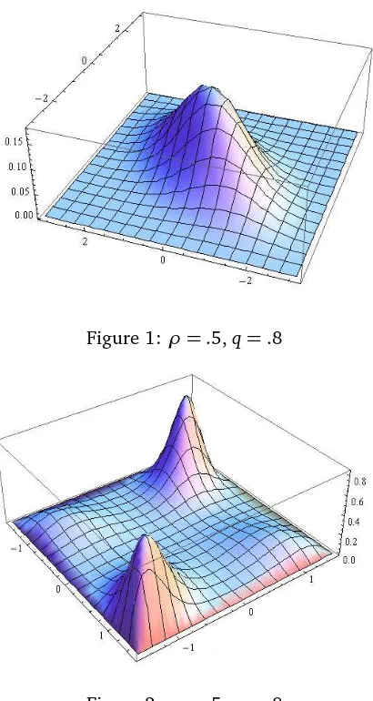
The simplest example of multidimensional density that can be constructed from these two distribu-tion is two dimensional density
g x,y|ρ,q
=fC N x|y,ρ,q
fN y|q
Figure 1: ρ=.5,q=.8
Figure 2: ρ=.5,q=.8
that will be referred to in the sequel asN2 0, 0, 1, 1,ρ|q
. Below we give some examples of plots of these densities. One can see from these pictures how large and versatile family of distributions is this family.
It has compact support equal to S q
×S q
and two parameters. One playing similar rôle to parameterρin two-dimensional Normal distribution. The other parameterqhas a different rôle. In particular it is responsible for modality of the distribution and of course it defines its support.
As stated above, distribution defined by fN x|q
theory.
The paper is organized as follows. In section 2 after recall some of the results ofq−series theory we present definition of multivariate q−Normal distribution. The following section presents main result. The last section contains lengthy proofs of the results from previous section.
2 Definition of multivariate
q
-Normal and some related distributions
2.1 Auxiliary results
We will use traditional notation of q−series theory i.e. [0]q = 0; [n]q = 1+q+. . .+qn−1 =
1−qn
1−q, [n]q! =
Qn
i=1[i]q, with [0]q! = 1,
n
k
q =
( [n]
q!
[n−k]q![k]q! , n≥k≥0
0 , other wise . It will be useful
to use so calledq−Pochhammer symbol forn≥ 1 : a|qn = Qni=0−11−aqi, with a|q0 = 1 ,
a1,a2, . . . ,ak|q
n=
Qk
i=1 ai|q
n. Often a|q
nas well as a1,a2, . . . ,ak|q
nwill be abbreviated to
(a)nand a1,a2, . . . ,ak
n, if it will not cause misunderstanding. It is easy to notice that q
n= 1−q
n
[n]q! and that
n
k
q =
(q)n
(q)n−k(q)k , n≥k≥0 0 , other wise
. The above mentioned quantities were defined for q < 1.
Note that forq=1[n]1=n,
n1
!=n!,(a|1)n= (1−a)nandn i
1=
n i
.
Let us also introduce two functionals defined on functions g:R−→C,
g
2
L=
Z
R
g(x)
2
fN(x)d x, g
2
C L=
Z
R
g(x)
2
fC N x|y,ρ,q
d x
and sets:
L q
= ¦g:R−→C:g
L<∞
©
,
C L y,ρ,q
= {g:R−→C:g
C L<∞}.
Spaces(L q,k.kL)and C L y,ρ,q,k.kC L
are Hilbert spaces with the usual definition of scalar product.
Let us also define the following two sets of polynomials:
-theq−Hermite polynomials defined by
Hn+1(x|q) =x Hn(x|q)−[n]qHn−1(x|q), (2.1)
forn≥1 withH−1(x|q) =0,H0(x|q) =1, and
-the so called Al-Salam-Chihara polynomials defined by the relationship forn≥0 :
Pn+1(x|y,ρ,q) = (x−ρyqn)Pn(x|y,ρ,q)−(1−ρ2qn−1)[n]qPn−1(x|y,ρ,q), (2.2)
withP−1 x|y,ρ,q
=0,P0 x|y,ρ,q
Polynomials (2.1) satisfy the following very useful identity originally formulated for so called contin-uousq−Hermite polynomialshn (can be found in e.g. [7]Thm. 13.1.5) and here below presented for polynomialsHn using the relationship
hn x|q
= 1−qn/2
Hn
2x
p
1−q|q
, n≥1, (2.3)
Hn x|q
Hm x|q
=
min(n,m)
X
j=0
m j
q
n j
q
j
q!Hn+m−2k x|q
. (2.4)
It is known (see e.g.[1]) thatq−Hermite polynomials constitute an orthogonal base of L q
while from[3] one can deduce that
Pn x|y,ρ,q n≥−1 constitute an orthogonal base of C L y,ρ,q
. Thus in particular 0=R
S(q)P1 x|y,ρ,q
fC N x|y,ρ,q
d x =E X|Y = y−ρy. Consequently, if
Y has alsoq−Normal distribution, thenEX Y =ρ.
It is known (see e.g.[7]formula 13.1.10) that
sup x∈S(q)
Hn x|q
≤Wn q
1−q−n/2
, (2.5)
where
Wn q
=
n
X
i=0
n
i
q
. (2.6)
We will also use Chebyshev polynomials of the second kind Un(x), that is Un(cosθ) =
sin(n+1)θ
sinθ
and ordinary (probabilistic) Hermite polynomials Hn(x) i.e. polynomials orthogonal with respect to p1
2πexp(−x
2/2). They satisfy 3
−term recurrences:
2x Un(x) = Un+1(x) +Un−1(x), (2.7)
x Hn(x) = Hn+1(x) +nHn−1 (2.8)
withU−1(x) =H−1(x) =0,U0(x) =H1(x) =1.
Some immediate observations concerningq-Normal and(y,ρ,q)−Conditional Normal distributions are collected in the following Proposition:
Proposition 1. 1. fC N x|y, 0,q
= fN(x|q).
2.∀n≥0 :Hn(x|0) =Un(x/2),Hn(x|1) =Hn(x).
3. ∀n ≥ 0 : Pn x|y, 0,q
= Hn(x|q), Pn(x|y,ρ, 1) = (1−ρ2)n/2Hn
x−ρy
p
1−ρ2
, Pn x|y,ρ, 0
=
Un(x/2)−ρy Un−1(x/2) +ρ2Un−2(x/2).
4. fN(x|0) = 1
2π
p
4−x2I<−2,2>(x), fN x|q
−→
q→1− 1 p
2πexp
−x2/2pointwise.
5. fC N x|y,ρ, 0
= (1−ρ
2)p4−x2
2π(1−ρ2)2−ρ(1+ρ2)x y+ρ2(x2+y2)I<−2,2>(x), fC N x|y,ρ,q
−→
q→1−
1
p
2π(1−ρ2)exp
−(x−ρy)
2
2(1−ρ2)
Proof. 1. Is obvious. 2. Follows observation that (2.1) simplifies to (2.7) and (2.8) forq=0 andq
=1 respectively. 3. First two assertions follow either direct observation in case ofPn x|y,ρ, 0
or comparison of (2.2) and (2.8) considered for x −→(x −ρy)/p1−ρ2 and then multiplication of
both sides by1−ρ2(n+1)/2
. Third assertion follows following observations: P−1 x|y,ρ, 0
=0,
P0 x|y,ρ, 0
=1,P1 x|y,ρ, 0
=x−ρy ,P2 x|y,ρ, 0
=x(x−ρy)−1−ρ2,Pn+1 x|y,ρ, 0
=x Pn x|y,ρ, 0
−Pn−1 x;y,ρ, 0
forn≥1 which is an equation (2.7) with x replaced by x/2.
4. 5. First assertions are obvious. Rigorous prove of pointwise convergence of respective densities can be found in work of[9]. To support intuition we will sketch the proof of convergence in distri-bution of respective distridistri-butions. To do this we apply 2. and 3. and see that∀n≥1Hn x|q
−→
Hn(x), and Pn(x|y,ρ,q)−→(1−ρ2)n/2Hn
x−ρy
p
1−ρ2
as q→1−. Now keeping in mind that
fam-ilies
Hn x|q n≥0 and
Pn x|y,ρ,q ≥0 are orthogonal with respect to distributions defined by respectively fN and fC N we deduce that distributions defined by fN and fC N tend to normalN(0, 1) andNρy,1−ρ2distributions weakly as q−→1− since both N(0, 1)andNρy,1−ρ2
are defined by their moments, which are defined by polynomialsHn, andPn.
2.2 Multidimensional
q
−
Normal and related distributions
Before we present definition of the multidimensional q−Normal and related distributions, let us generalize the two discussed above one-dimensional distributions by introducing(m,σ2,q)−Normal distribution as the distribution with the density fN((x−m)/σ|q)/σform∈R,σ >0,q∈(−1, 1]. That is ifX ∼(m,σ2,q)−Normal then(X−m)/σ∼q−Normal.
Similarly let us extend definition of(y,ρ,q)−Conditional Normal by introducing form∈R,σ >0,
q ∈ (−1, 1], ρ
< 1, (m,σ2,y,ρ,q)-Conditional Normal distribution as the distribution whose
density is equal to fC N (x−m)/σ|y,ρ,q
/σ.
Letm,σ∈Rd andρ∈(−1, 1)d−1,q∈(−1, 1]. Now we are ready to introduce a multidimensional
q−Normal distributionNd
m,σ2,ρ|q
.
Definition 1. Multidimensionalq−Normal distributionNdm,σ2,ρ|q
, is the continuous distribu-tion inRd that has density equal to
gx|m,σ2,ρ,q
= fN
(x
1−m1 σ1
|q
d−1 Y
i=1
fC N
x
i+1−mi+1 σi+1
|xi−mi
σi
,ρi,q
/
d
Y
i=1 σi
wherex= x1, . . . ,xdd
,m= m1, . . . ,md
,σ2=
σ21, . . . ,σ2d,ρ= (ρ1, . . . ,ρd−1).
As an immediate consequence of the definition we see that supp(Nd(m,σ2|q)) = m+S q. One
can also easily see that m is a shift parameter and σ is a scale parameter. Hence in particular
EX=m. In the sequel we will be mostly concerned with distributionsNd(0,1,ρ|q).
Remark1. Following assertion 1. of Proposition 1 we see that distributionNd 0,1,0|q
is the prod-uct distribution of d i.i.d. q−Normal distributions. Another words "lack of correlation means in-dependence" in the case of multidimensional q−Normal distributions. More generally if the se-quenceρ= (ρ1, . . . ,ρd−1)contain, say, r zeros at, say, positions t1, . . . ,tr then the distribution of
Nd 0,1,ρ
is a product distribution ofr+1 independent multidimensionalq−Normal distributions:
Nt1
0,1,(ρ1, . . . ,ρt
1−1)
, . . . ,Nd−tr
0,1,(ρt
r+1, . . . ,ρtd
Thus in the sequel all considered vectorsρwill be assumed to contain only nonzero elements.
Let us introduce the following functions (generating functions of the families of polynomials):
ϕ x,t|q
= ∞
X
i=0
ti
[i]q!Hi x|q
, (2.9)
τ x,t|y,ρ,q
= ∞
X
i=0
ti
[i]q!Pi x|y,ρ,q
. (2.10)
The basic properties of the discussed distributions will be collected in the following Lemma that contains facts from mostly[7]and the paper[3].
Lemma 1. i) For n,m≥0 :
Z
S(q)
Hn x|q
Hm x|q
fN x|q
d x=
¨
0 when n6=m
[n]q! when n=m .
ii) For n≥0 :
Z
S(q)
Hn x|q
fC N x|y,ρ,q
d x =ρnHn y|q
.
iii) For n,m≥0 :
Z
S(q)
Pn x|y,ρ,q
Pm x|y,ρ,q
fC N x|y,ρ,q
d x=
¨
0 when n6=m
ρ2
n[n]q! when n=m .
iv)
Z
S(q)
fC N x|y,ρ1,q
fC N y|z,ρ2,q
d y= fC N x|z,ρ1ρ2,q
.
v) For|t|,q <1 :
∞
X
i=0
Wi q
ti q
i
= 1 (t)2∞,
∞
X
i=0
Wi2 q
ti
q
i
=
t2
∞ (t)4∞ ,
convergence is absolute, where Wi q
is defined by (2.6).
vi) For(1−q)x2≤2and∀(1−q)t2<1 :
ϕ x,t|q
= ∞
Y
k=0
1− 1−q
x tqk+ 1−q
t2q2k−1,
convergence (2.9) is absolute in t & x and uniform in x. Moreover ϕ x,t|q
is positive and
R
S(q)ϕ x,t|q
fN x|q
d x=1. ϕ(t,x|1) =expx t−t2/2.
vii) For(1−q)max(x2,y2)≤2,ρ
<1and∀(1−q)t2<1 :
τ x,t|y,ρ,q
= ∞
Y
k=0
1− 1−qρy tqk+ 1−qρ2t2q2k
1− 1−q
x tqk+ 1−q
convergence (2.10) is absolute in t & x and uniform in x. Moreover τ x,t|θ,ρ,q
is positive and
R
S(q)τ x,t|y,ρ,q
fC N x|y,ρ,q
d x=1.
τ x,t|y,ρ, 1
=expt x−ρy
−t2(1−ρ2)/2.
viii) For(1−q)max(x2,y2)≤2,ρ <1 :
fC N x|y,ρ,q
= fN x|q
∞
X
n=0 ρn
[n]q!Hn(x|q)Hn(y|q) (2.11)
and convergence is absolute t, y & x and uniform in x and y.
Proof. i) It is formula 13.1.11 of [7] with obvious modification for polynomials Hn instead ofhn
(compare (2.3)) and normalized weight function (i.e. fN) ii) Exercise 15.7 of[7]also in [1], iii) Formula 15.1.5 of [7] with obvious modification for polynomials Pn instead of pn x|y,ρ,q
=
(1−q)n/2P
2x
p1
−q|
2y
p1
−q,ρ,q
and normalized weight function (i.e. fC N), iv) see (2.6) of[3]. v)
Exercise 12.2(b) and 12.2(c) of[7]. vi)-viii) The exact formulae are known and are given in e.g.
[7](Thm. 13.1.1, 13.1.6) and[10](3.6, 3.10). Absolute convergence ofϕ andτfollow (2.5) and v). Positivity ofϕ andτfollow formulae 1− 1−q
x tqk+ 1−q
t2q2k= (1−q)(tqk−x/2)2+
1−(1−q)x2/4 and 1− 1−q
ρy tqk+ 1−q
ρ2t2q2k= (1−q)ρ2(qkt−y/(2ρ))2+1−(1−q)y2/4. Values of integrals follow (2.9) and (2.10) and the fact that
Hn and
Pn are orthogonal bases in spacesL q
andC L y,ρ,q
.
Corollary 1. Every marginal distribution of multidimensional q−Normal distribution Ndm,σ2,ρ|q
is multidimensional q−Normal. In particular every one-dimensional distribution is q−Normal. More precisely i−th coordinate of Nd
m,σ2,ρ|q
−vector has(mi,σ2i,q)−Normal distribution.
Proof. By considering transformation(X1, . . . ,Xd)−→(X1−m1
σ1 , . . . ,
Xd−md
σd )we reduce considerations
to the caseNd 0,1,ρ|q. First let us considerd−1 dimensional marginal distributions. The
asser-tion of Corollary is obviously true since we have asserasser-tion iv) of the Lemma 1. We can repeat this reasoning and deduce that all d−2, d−3, . . . , 2 dimensional distributions are multidimensional
q−Normal. The fact that 1−dimensional marginal distributions areq−normal follows the fact that
fC N y|x,ρ,q
is a one-dimensional density and integrates to 1.
Corollary 2. IfX= (X1, . . . ,Xd)∼Nd m,1,ρ|q
, then
i)∀n∈N, 1≤ j1< j2. . .< jm<i≤d:
Xi|Xjm, . . . ,Xj1∼ fC N
xi|xjm,Qik−=1j
mρk,q
.Thus in particular
EHn Xi−mi|Xj
1, . . . ,Xjm
=
i−1
Y
k=jm ρk
n
HnXjm−mjm
andvarXi|Xj
1, . . . ,Xjm
=1−Qik−=1j
mρk
2
.
ii)∀n∈N, 1≤ j1<. . .jk<i< jm<. . .< jh≤d:
Xi|Xj
1, . . .Xjk,Xjm, . . . ,Xjh∼ fN xi|q
∞
Y
l=0
hlxjk,xjm,ρ∗kρ∗m,q hl(xi,xjk,ρ∗
k,q)hl(xi,xjm,ρ ∗
where hl x,y,ρ,q
= ((1−ρ2q2l)2−(1−q)ρql1+ρ2q2lx y + (1−q)ρ2q2l(x2+ y2)), ρ∗k =
Qi−1
i=jkρi,ρ ∗
m=
Qjm−1
i=i ρi. Thus in particular this density depends only on Xjk and Xjm.
Proof. i) As before, by suitable change of variables we can work with distribution Nd 0,1,ρ|q.
Then following assertion iii) of the Lemma 1 and the fact that m− dimensional marginal, with respect to which we have to integrate is also multidimensionalq−Normal and that the last factor in the product representing density of this distribution is fC N
xi|xjm,
Qi−1
k=jmρk,q
we get i).
ii) First of all notice that joint distribution of(Xj1, . . .Xjk,Xi,Xjm, . . . ,Xjh)depends only onxjk,xi,xjm
since sequenceXi,i=1 . . . ,nis Markov. It is also obvious that the density of this distribution exist and can be found as a ratio of joint distribution of Xj
k,Xi,Xjm
divided by the joint density of
Xj
k,Xjm
. Keeping in mind thatXj
k,Xi,Xjm have the same marginalfN and because of assertion iv
of Lemma 1 we get the postulated form.
Having Lemma 1 we can present Proposition concerning mutual relationship between spacesL q
andC L y,ρ,q
defined at the beginning of previous section.
Proposition 2. ∀q ∈ (−1, 1),y ∈ S q
,ρ
< 1 : L q
= C L y,ρ,q
. Besides ∃C1 y,ρ,q
,
C2 y,ρ,q
:g
L≤C1
g
C L and
g
C L≤C2
g
L for every g∈L q
.
Proof. Firstly observe that : (1−ρ2q2k)2−(1−q)ρqk(1+ρ2q2k)x y + (1−q)ρ2(x2+ y2)q2k =
(1−q)ρ2q2kx−yρqk+ρ2−1q−k2+ (1−(1−q)y2/4)(1−ρ2q2k)2 which is elementary to prove. We will use modification of the formula (2.11) that is obtained from it by dividing both sides by
fN x|q
. That is formula:
∞
Y
k=0
1−ρ2qk
(1−ρ2q2k)2−(1−q)ρqk(1+ρ2q2k)x y+ (1−q)ρ2(x2+y2)q2k
= ∞
X
n=0 ρn
[n]q!Hn x|q
Hn y|q
.
Now we use (2.5) and assertion v) of Lemma 1 and get∀x,y∈S q
:
fC N x|y,ρ,q
≤ fN x|q
ρ2∞ ρ4
∞
.
HenceC2=
(ρ2)
∞
(ρ)4∞ and
g
2
C L≤
g
2
L, for everyg∈L q
. Thus g∈C L y,ρ,q.
Conversely to take a function g∈C L y,ρ,q
. We have
∞>
Z
S(q)
g(x)
2
fC N x|y,ρ,q
d x.
Now we keeping in mind that(1−ρ2q2k)2−(1−q)ρqk(1+ρ2q2k)x y+ (1−q)ρ2(x2+ y2)q2k is a quadratic function inx, we deduce that it reaches its maximum for x∈S q
S q
and we see that
∞>
Remark2. Notice that the assertion of Proposition 2 is not true forq=1 since then the respective densities areN(0, 1)andNρy, 1−ρ2.
Remark 3. Using assertion of Proposition 2 we can rephrase Corollary 2 in terms of contraction
R ρ,q
defined by the formula (using polynomialsHn
forρ
By the way it is known thatR is not only contraction but also ultra contraction i.e. mapping L2 on
L∞(Bo˙zejko).
We have also the following almost obvious observation that follows, in fact, from assertion iii) of the Lemma 1.
Proposition 3. Suppose thatX=(X1, . . . ,Xd)∼Nd 0,1,ρ|q
and g ∈ L q
. Assume that for some n∈N,and1≤ j1< j2. . .< jm<i≤d.
i) IfEg Xi|Xj
1, . . . ,Xjm
=polynomial of degree at most n of Xjm,then function g must be also a
ii) If additionallyEg Xi=0
E((E(g(Xi)|Xj
1, . . . ,Xjm) 2)
≤r2Eg2(Xi), (Generalized Gebelein’s inequality)
where r=Qik−=1j
mρk.
Proof. i) The fact that Eg Xi|Xj
1, . . . ,Xjm
is a function of Xj
m only, is obvious. Since g ∈
L q
we can expand it in the series g(x) = Pi≥0ciHi x|q
. By Corollary 2 we know that
Eg Xi|Xj
1, . . . ,Xjm
= Pi≥0ciriHXj
m|q
for r = Qik−=1j
mρk. Now since cir
i = 0 for i > n andr6=0 we deduce thatci =0 fori>n.
ii) Suppose g(x) = P∞i=1giHi(x). We have E(g(Xi)|Xj1, . . . ,Xjm) =
P∞
i=1giriHi(Yjm). Hence
E((E(g(Xi)|Xj
1, . . . ,Xjm)
2) =P∞
i=1g 2
i r
2i[i] q!≤r2
P∞
i=1g 2
i [i]q!=r2Eg2(Xi).
Remark4. As it follows from the above mentioned definition, the multidimensionalq−Normal dis-tribution is not a true generalization of n−dimensional Normal lawNn(m,˚). It a generalization of distributionNn(m,˚) with very specific matrix ˚namely with entries equal to σii = σ2i;σi j =
σiσj
Qj−1
k=iρk fori< j andσi j =σji fori> j whereσi ; i=1, . . . ,nare some positive numbers andρi
<1,i=1, . . . ,n−1.
Proof. Follows the fact that two dimensionalq−Normal distribution of sayXi/σi,Xj/σj
has
den-sity fN xi|q
fC N
xj|xi,Qkj−=1iρk,q
ifi< j.
Remark 5. Suppose that(X1, . . . ,Xn)∼ Nn m,σ,ρ|qthen X1, . . . ,Xn form a finite Markov chain
withXi ∼(mi,σ2i,q)−Normal and transition densityXi|Xi−1= y ∼(mi,σ2i,y,ρi−1,q)-Conditional
Normal distribution
Following assertions vi) and vii) of Lemma 1 we deduce that for∀t2<1/(1−q),ρ
<1 functions
ϕ x,t|q
fN x|q
andτ x,t|y,ρ,q
fC N x|y,ρ,q
are densities. Hence we obtain new densities with additional parameter t. This observation leads to the following definitions:
Definition 2. Let q
∈ (−1, 1],t2 < 1/(1−q),x ∈ S q. A distribution with the density
ϕ x,t|q
fN x|q
will be calledmodified t,q
−Normal (briefly t,q
−MN distribution).
We have immediate observation that follows from assertion vi) of Lemma 1.
Proposition 4. i)R
S(q)ϕ y,t|q
fN y|q
fC N x|y,ρ,q
d y=ϕ x,tρ|q
fN(x|q)
ii) Let X ∼ t,q
−MN. Then for n∈N:E Hn X|q=tn.
Proof. i) Using assertions vi) and viii) of the Lemma 1 we get:
Z
S(q)
ϕ y,t|q
fN y|q
fC N x|y,ρ,q
d y
= fN x|q
Z
S(q)
fN y|q
∞
X
i=1
ti
[i]q!Hi y|q
∞
X
j=0 ρj
[j]q!Hj y|q
Hj x|q
Now utilizing assertion ii) of the same Lemma we get:
Z
S(q)
ϕ y,t|q
fN y|q
fC N x|y,ρ,q
d y
= fN x|q
∞
X
i=0
tρi
[i]q! Hi x|q
=ϕ x,tρ|q
fN(x|q).
To get ii) we utilize assertion vi) of the Lemma 1.
In particular we have:
Corollary 3. If X∼(t,q)−M N , thenEX=t, var(X) =1,E(X−t)3=−t 1−q,E(X−t)4=
2+q−t25+6q+q2.
Proof. We have x3 = H3 x|q
+ 2+q
H1(x) and H4 x|q
+ (3+2q+q2)H2 x|q
+2+q =
x4soE(X−t)3=EX3−3EX2t+3E(X)t2−t3=t3+ 2+qt−3t1+t2+3t3−t3= −t 1−q
andE(X−t)4=EX4−4tEX3+6t2EX2−4t3E(X)+t4=t4−(3+2q+q2)t2+
2+q−4tt3+ 2+q
t+6t2t2+1−4t4+t4which reduces to 2+q−t25+6q+q2.
In particular kurtosis of t,q
−M N distributions is equal to− 1−q
−t25+6q+q2. Hence it is negative and less, fort6=0, than that ofq−Normal which is also negative (equal to− 1−q
).
Assertion i) of the Proposition 4 leads to the generalization of the multidimensional q−Normal distribution that allows different one-dimensional and other marginals.
Definition 3. A distribution inRd having density equal to
ϕ x1,t|q
fN x1|q
d−1
Y
i=1
fC N xi+1|xi,ρi,q
,
where xi ∈S q
, ρi ∈(−1, 1)\ {0}, i= 1, . . . ,d−1, q
∈(−1, 1], t2 <1/(1−q)will be called
modified multidimensional q-Normal distribution(brieflyM M Nd(ρ|q,t)).
Reasoning in the similar way as in the proof of Corollary 1 and utilizing observation following from Proposition 4, we have immediately the following observation.
Proposition 5. Let(X1, . . . ,Xd)∼M M Nd(ρ|q,t). Then every marginal of it is also modified multidi-mensional q−Normal. In particular∀i=1, . . . ,d :Xi∼tQik−=11 ρk,q
−M N
Remark6. Suppose that(X1, . . .Xd)∼M M Nd(ρ|q,t)and defineρ0=1, then the sequenceX1, . . .Xd
form a non-stationary Markov chain such thatXi ∼ϕ
x|tQik−=11ρk,q
fN x|q
with transitional probabilityXi+1|Xi= y∼ fC N x|y,ρi,q
.
Definition 4. Letq
∈(−1, 1],t2<1/(1−q),x,y ∈S q
,ρ
<1. A distribution with the
den-sity τ x,t|y,ρ,qfC N x|y,ρ,q
will be called modified y,ρ,t,q−Conditional Normal (briefly
y,ρ,t,q
−MCN).
We have immediate observation that follows from assertion vii) of Lemma 1.
Proposition 6. Let X ∼ y,ρ,t,q
−MCN. Then for n∈N:E Pn X|y,ρ,q=ρ2
nt n.
Hence in particular one can state the following Corollary.
Corollary 4. EX =ρy+ (1−ρ2)t, var(X) = (1−ρ2)(1−(1−q)t yρ+ (1−q)t2ρ2).
Proof. Follows expressions for first two Al-Salam-Chihara polynomials. Namely we have:
P1(x|y,ρ,q) =x−ρy, P2(x|y,ρ,q) =x2−1+ρ2+qρ2y2−xρy(1+q).
We can define two formulae for densities of multidimensional distributions inRd. Namely one of
them would have density of the form
ϕ x1,t|q
fN x1|q
τ x2,t|x1,ρ1,q
d−1
Y
i=1
fC N xi+1|xi,ρi,q
and the other of the form
fN x1|q
τ x2,t|x1,ρ1,q
d−1
Y
i=1
fC N xi+1|xi,ρi,q
.
However to find marginals of such families of distributions is a challenge and an open question. In particular are they also of modified conditional normal type?
3 Main Results
In this section we are going to study properties of 3 dimensional case of multidimensional normal distribution. To simplify notation we will consider vector (Y,X,Z) having distribution
N3((0, 0, 0),(1, 1, 1),(ρ1,ρ2)|q) that is having density fC N y|x,ρ1,q
fC N(x|z,ρ2,q)fN(z|q). We start with the following obvious result:
Remark7. Conditional distributionX|Y,Z has density
φ x|y,z,ρ1,ρ2,q
= fN x|q
ρ21,ρ22 ∞
ρ21ρ22∞ ∞
Y
i=0
wk y,z,ρ1ρ2,q
wk x,y,ρ1,q
wk x,z,ρ2,q
, (3.1)
where we denotedwk s,t,ρ,q
= (1−ρ2q2k)2−(1−q)ρqk(1+ρ2q2k)st+ (1−q)ρ2(s2+t2)q2k.
Remark 8. Notice that φ x|y,z,ρ1,ρ2,q
is the re-scaled Askey-Wilson density. Namely
φ x|y,z,ρ1,ρ2,q function of Askey-Wilson polynomials. Compare e.g.[5]and[7]. Hence our results would concern properties of Askey - Wilson density and Askey-Wilson polynomials.
Let us denote
Remark 9. Following probabilistic interpretation of function gn (as conditional expectation) and (2.5) we deduce that forq
<1,y,z∈S q
gn y,z,ρ1,ρ2,q≤Wn q 1−q−n/2. (3.2)
Our main result is the following
Theorem 1. i)φ x|y,z,ρ1,ρ2|q
is a polynomial in y of order k and
in z of order l. MoreoverΘ0,n y,z, 0|q
=Hn z|q
andΘn,0 y,z, 0,q
=Hn y|q
.
Remark10. Assertion i) of the Theorem 1 is in fact a generalization of Poisson-Mehler formula (that is assertion viii) of Lemma 1) for Askey-Wilson density.
Remark 11. Notice also that for q = 1, φ is a density function of normal distribution
N
and it is obvious that expectation of any polynomial is a
polynomial in yρ1(1−ρ22)+zρ2(1−ρ21)
1−ρ2 1ρ22
. Hence it turns out that this is true for all q−Normal distribu-tions forq∈(−1, 1].
As a Corollary we have the following result.
Corollary bellow gives detailed form of coefficientsA(rn,s)forn=1, . . . , 4.
Remark12. Notice that in general conditional variance var Xi|X1, . . . ,Xi−1,Xi+1, . . . ,Xd
is not nonrandom indicating that q−Normal distribution does not behave as Normal in this case, however if we set q = 1 in (3.4) then we get
as it should be in the normal case.
Notice that examining the form of coefficientsA(mn,)kforn=1, . . . , 4 we can formulate the following Hypothesis concerning general form of them:
Conjecture 1. For n≥1, we have: A(0,n−⌊) n/2⌋+l =n polynomial in q with coefficients depending only on r and l.
4 Proofs
. We will need some of its properties. Namely we will prove
the following Proposition which is in fact a generalization and reformulation (in terms of polyno-mials Hn) of an old result of Carlitz. Original result of Carlitz concerned polynomials wn(x|q) =
Pn
i and expressions of the form P∞
iii)
Gk,0 y,z,t|q
=
k
X
i=0
(−1)i
k
i
q
q(2i)tiHk
−i(y|q)G0,i(y,z,t|q). (4.2)
iv)
Gk,0 y,z,t|q
= 1
1−qk(k−1)t2k
k−1
X
i=0
(−1)iq(2i)
k
i
q
tiτk,i y,z,t|q
, (4.3)
whereτk,i y,z,t|q
= (Hk−i(y|q)G0,i(y,z,t|q) + (−1)kq(
k
2)tkHk
−i(z|q)Gi,0(y,z,t|q)).
Proof. i) is obvious.
iii) Take j=kandl =0 in ii).
ii) To prove (4.1) we will use formula
Hn+m x|q
=Hn x|q
Hm(x|q)−
Pmin(n,m)
j=1
n j
q
m j
q
jq!Hn+m−2j(x|q). We have
Gk,l y,z,t
= X
m≥0
tm
[m]q!Hm+k y|q
Hm+l z|q
=X
m≥0
tm
[m]q!(Hk y|q
Hm(y|q)
−
min(k,m)
X
j=1
k
j
q
m
j
q
j
q!Hk+m−2j(y|q))Hm+l z|q
=Hk y|q
G0,l(y,z,t)−
k
X
j=1
tj
k j
q
∞
X
m=j
tm−j
m−j
q!
Hk+(m−j)−j(y|q)Hl+j+(m−j)(z|q)
=Hk y|q
G0,l(y,z,t)−
k
X
j=1
tj
k
j
q
Gk−j,l+j(y,z,t).
formula (forGk,l)applied fork−>k−mandl−>m+l:
iv) Fork=0 this is obviously true. Now let us iterate (4.2) once, applied however, forG0,k. We will get then
Now we are ready to present the proof if Theorem 1.
Proof of the Theorem 1. First notice that following (3.2) and assertion v of Lemma 1 we see that
seriesPn≥0Hn(x|q)gn(y,z,ρ1,ρ2,q)
1, that is Poisson-Mehler expansion formula. Following (3.1) we see that
First, let us concentrate on the quantity:
R x,y,z,ρ1,ρ2|q
. Our Theorem will be
proved if we will be able to show that ∀l,k ≥ 0 : Gl,k y,z,t|q
= G0,0 y,z,t|q
Θl,k y,z,t|q
whereΘl,kis a polynomial of order al in y kinz. This fact follows by induction from formula (4.3) of assertion iv) of the Proposition 7 since it expresses Gk,0 in terms of kfunctions Gi,0 andG0,i for
i=0, . . . ,k−1 and the fact that allGl,k can be expressed byGi,0andG0,i ;i≤k+l.
Proof of Corollary 5. By Theorem 1 we know that regression
E(Hn Xi|q|Xj
of both sides. On one hand we get
EHn Xi|q|Xj
on the other we get
n
Thus we have equality:
Now we use the identity (2.4) and get