23 11
Article 09.1.7
Journal of Integer Sequences, Vol. 12 (2009), 2
3 6 1 47
Polygonal Chain Sequences
in the Space of Compact Sets
Steven Schlicker
Grand Valley State University
Allendale, MI 49401
USA
Lisa Morales
University of California, Riverside
Riverside, CA 92521
USA
Daniel Schultheis
University of California, San Diego
La Jolla, CA 92093
USA
Abstract
Configurations in the hyperspace of all non-empty compact subsets ofn-dimensional
real space provide a potential wealth of examples of familiar and new integer sequences. For example, Fibonacci-type sequences arise naturally in this geometry. In this paper, we introduce integer sequences that are determined by polygonal chain configurations.
1
Introduction
geometry on H(Rn), the hyperspace of all non-empty, compact subsets of Rn. The concept
of betweenness in this geometry gives rise to interesting examples of integer sequences. In this context we will introduce polygonal chains and new integer sequences related to them. Throughout this article, we let Fk denote the kth Fibonacci number (with F0 = 0, F1 = 1)
and Lk the kth Lucas number (with L0 = 2, L1 = 1). Recall that the Lucas numbers Lk
satisfy
Lk =Fk−1+Fk+1 = 2Fk−1 +Fk.
2
The Hausdorff Metric
The Hausdorff metrichwas introduced by Felix Hausdorff in the early 20th century as a way to measure the distance between compact sets. The Hausdorff metric imposes a geometry on the space H(Rn), which will be the subject of our study. To distinguish between Rn and
H(Rn), we will refer to points in Rn and elements inH(Rn).
Definition 1. Let A and B be elements in H(Rn). The Hausdorff distance, h(A, B), between A and B is
h(A, B) = max{d(A, B), d(B, A)},
where d(A, B) = maxa∈A{d(a, B)} and d(a, B) = minb∈B{dE(a, b)}.
As an example, let A be the two point set {(−1,0),(1,0)} and B the circle centered at (0,0) of radius 1 in R2. Since A ⊂ B, we have d(A, B) = 0. However, d(B, A) =
dE((0,1),(1,0)) =
√
2. Note that d(A, B) 6= d(B, A), so the function d is not symmetric. That is why we need the maximum of d(A, B) and d(B, A) to obtain a metric. In our example, we haveh(A, B) = d(B, A) =√2. See Barnsley [1] for a proof thathis a metric on H(Rn). The corresponding metric space, (H(Rn), h), is then itself a complete metric space
[1].
3
Betweenness in
H
(
R
n)
Betweenness will play a major role in this paper, allowing us to find new integer sequences. In this section we define “betweenness” in H(Rn), mimicking the idea of betweenness in Rn
under the Euclidean metric. It is in this context that we will later define polygonal chains and introduce an infinite family of new integer sequences. Before we discuss betweenness, we define the dilation of a set, which will play a critical role in what follows.
Definition 2. Let A∈ H(Rn) and let s >0 be a real number. The dilation of A bys is the set
(A)s={x∈Rn:dE(x, a)≤s for some a∈A}.
As a simple example, the dilation of a single point set A = {a} by s is the closed ball centered at a of radius s. In general, the s-dilation of the set A is the union of all closed
A
A B
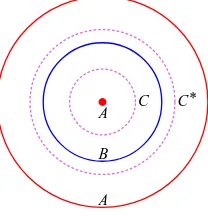
[image:3.612.260.364.39.147.2]C C*
Figure 1: Infinitely many elements at the same location betweenAandB.
An important and useful result about dilations is the following (Theorem 4 from the article [6]).
Theorem 3. Let A∈ H(Rn) and lets >0. Then (A)s is a compact set withh(A,(A)s) =s. Moreover, if C ∈ H(Rn) and h(A, C)≤s, then C ⊆(A)s.
In other words, the element (A)sis the largest element (in the sense of containment) that
is a distance s from A. Now we discuss betweenness. In the standard Euclidean geometry, a point x lies between the points a and b if and only if dE(a, b) = dE(a, x) +dE(x, b). We
extend this idea to H(Rn).
Definition 4. Let A, B ∈ H(Rn) with A =6 B. The element C ∈ H(Rn) lies between A
and B if h(A, B) = h(A, C) +h(C, B).
Notation: We write ACB to signify that C is between A and B as in Blumenthal [5]. Betweenness in Rn is quite different than betweenness in H(Rn). Consider the following
examples.
Example 5. Let A the union of the origin with the circle centered at (0,0) with radius 10 and B the circle centered at (0,0) with radius 5 in H(R2) as shown in Figure 1. Then
h(A, B) =d(A, B) =d(B, A) = 5. The unionC∪C∗ of the two dashed circles is the element (A)2∩(B)3. Theorem 3 shows that any element X satisfying AXB with h(A, X) = s and
h(B, X) = h(A, B)−s must be a subset of (A)s ∩(B)h(A,B)−s. It is not difficult to see
that if Xc = {c} ∪C∗ where c is any point on the circle C, then X satisfies AXB with
h(A, X) = 2. So in this example, there are infinitely many different elements X satisfying
AXB and h(A, X) = 2.
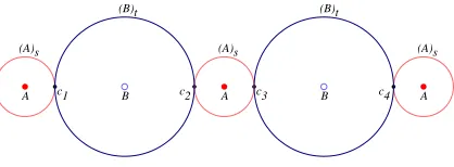
Example 6. LetA ={(−2,0),(0,0),(2,0)} and B ={(−1,0),(1,0)} inR2 as shown in
Figure2. Let 0< s < h(A, B) and lett=h(A, B)−s. In this case, the setC = (A)s∩(B)t
is the four point set C ={c1, c2, c3, c4}. Since any elementC′ that lies between A and B at
the distance s fromA is a subset of C, there are at most 16 elements C′ that could satisfy
AC′B with h(A, C′) =s. However, not every subset of C has this property. For example, if
C′ ={c1}, thenh(A, C′) = 3 +t andC′ does not satisfy AC′B. We leave it to the reader to
show that the setsC, {c1, c2, c4}and {c1, c3, c4} are the only sets that lie between A and B
A c1 B c2 A c3 B c4 A
(A)s (A)s (A)s
[image:4.612.208.417.35.112.2](B)t (B)t
Figure 2: Exactly 3 different elements at the same location betweenAandB.
between two fixed elements at a specific distance from one of them that will be of interest to us.
The next definition formalizes what is meant when we refer to two elements at thesame location between sets A and B.
Definition 7. Let A, B ∈ H(Rn) with A =6 B and let C, C′ ∈ H(Rn) satisfy ACB
and AC′B. The elements C, C′ are said to be at the same location between A and B if
h(A, C) =h(A, C′) = s for some 0< s < h(A, B).
4
Finding Points Between
A
and
B
LetA, B ∈ H(Rn). If a setC ∈ H(Rn) satisfiesACB withh(A, C) = s, then it follows from
Theorem 3that C ⊆(A)s∩(B)h(A,B)−s. As we saw in Examples5and 6, for some elements
Aand B there are infinitely many different elements at the same location betweenA and B
and for other A and B there are only finitely many elements at the same location between them. The latter situation is of interest to us. In article [4], the authors show that in order for a pair of elements A and B inH(Rn) to have a finite number of elements inH(Rn) at a
given location betweenA and B, every point inA must be a common distance r=h(A, B) away from B (that is, d(a, B) = r for all a ∈ A) and every point in B must be that same distance r from A (d(b, A) = r for all b ∈ B). If this condition is not met, there will be infinitely many elements in H(Rn) at each location betweenA and B. If a pair of elements
A, B ∈ H(Rn) satisfies this condition, we call the pair a configuration.
Definition 8. A finite configuration is a pair [A, B] of finite sets A, B ∈ H(Rn) where
d(a, B) = d(b, A) =h(A, B) for all a∈A and b∈B.
In article [4], the authors also show that if [A, B] is a finite configuration, then the number of elements C satisfying ACB and h(A, C) = s is independent of s for all 0 < s < h(A, B). Thus, we denote by #([A, B]) the number of elements betweenA and B in a finite configuration [A, B] at any distance s.
Note that if [A, B] is a finite configuration, then C = (A)s∩(B)h(A,B)−s will be a finite
Figure 3: TheP4configuration.
5
String and Polygonal Configurations
Two basic configurations that will be relevant to our work are string and polygonal config-urations. A string configuration is any finite set of points equally spaced on a line segment, with sets A and B consisting of alternate points on the line [9]. Figure 2 is an example. If |A∪B|=k, then we will call the string configuration [A, B] a k−string and denote it as
Sk. So Figure 2shows a 5-string or S5. In article [9] (Theorem 6.1) the authors show
#(Sk) = Fk−1.
In Figure 2, the elements {c1, c2, c3, c4},{c1, c2, c4}, and {c1, c3, c4} are the elements that
satisfy ACB at the indicated location in this example. This is as expected, since #(S5) =
F4 = 3.
Another basic family of configurations is the collection of polygonal configurations. LetA
andB be the alternate vertices of a regular 2m-gon withm ∈N. We denote the configuration
[A, B] in this case by Pm and call this a polygonal configuration [9]. An example of P4 is
shown in Figure3, with the set Aas the filled points and the set B as the open points. Line segments are drawn between points to indicate the pairs of pointsa∈Aandb∈B satisfying
dE(a, b) =h(A, B). These points will be important in what follows.
Definition 9. Let [A, B] be a finite configuration. The points a ∈ A and b ∈ B are
adjacent if dE(a, b) = h(A, B). If a ∈ A, the adjacency set of a, [a]B, is defined as [a]B =
{b∈B :dE(a, b) = h(A, B)}.
Again in the paper [9] (Theorem 6.3) the authors show
#(Pm) =F2m+ 2F2m−1 =L2m.
String and polygonal configurations form the building components of polygonal chains.
6
Polygonal Chains
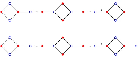
A polygonal chainP Ck
m,lis a configuration obtained by connectingkcopies ofPmat antipodal
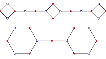
points with string configurations of a fixed length l+ 1. When k = 1, we define P Cm,l1 to be Pm. Examples of polygonal chains are shown in Figure 4. In this section we determine
Figure 4: Top:P C3
2,3 Bottom:P C 2 3,2.
6.1
Adjoining Configurations
To compute #(P Cm,lk ), we will ultimately reduce the problem to one of determining #(X) for smaller configurations X created from adjoins of polygonal and string configurations. Before discussing adjoins, we need to understand equivalent configurations. The idea here is that in the computation of #([A, B]) the distance between adjacent points is irrelevant -only adjacencies matter.
Definition 10. The finite configuration [X, Y] is equivalent to the finite configuration [A, B] if there are bijections f : A →X and g : B →Y such that for all a ∈A and b ∈ B, we have a adjacent to b if and only iff(a) is adjacent to g(b). When [X, Y] is equivalent to [A, B] we write [X, Y]∼[A, B].
It is easy to show that the relation ∼ is an equivalence relation on the set of finite configurations. One important result involving equivalent configurations is that if [X, Y] and [A, B] are equivalent configurations, then #([X, Y]) = #([A, B]) [4] (Theorem 4.1). Now we adjoin a point to a configuration.
Definition 11. Let [A, B] be a finite configuration. The configuration [A, B](a, y) ob-tained by adjoining a point y 6∈ A ∪B to [A, B] at the point a ∈ A is the configuration [A, B′], where B′ =B∪ {y}, dE(y, a) = h(A, B), and dE(y, x) > h(A, B) for all x∈ A∪B with x6=a.
For example, Figure 5 shows the configuration obtained by adjoining a point y to P4 at
point a.
One tool for computing #([A, B](a, y)) for a finite configuration [A, B] is the following [9] (Theorem 6.2).
a y
[image:6.612.270.352.568.630.2]a y c0
Figure 6: AdjoiningP2andP3.
Theorem 12. Let [A, B] be a finite configuration. Define a new configuration X′ by adjoin-ing a pointy to [A, B] at the point a∈A. Furthermore, assume a is adjacent tok points in
B, each of which is adjacent to at least one more point in A. Then
#(X′) = #([A, B]) + #([A− {a}, B]).
As an example, if [A, B] =P4 and X′ = [A, B](a, y) as shown in Figure 5, then #(X′) =
#(P4) + #(S7) = L8+F6 = 55.
We can also adjoin two configurations.
Definition 13. Let [A, B] and [X, Y] be finite configurations and let a∈ A and y∈ Y. Let [X′, Y′] be a configuration equivalent to [X, Y] through bijections f : X → X′ and
g :Y →Y′ so that
1. h(X′, Y′) =h(A, B),
2. dE(g(y), a) = h(A, B),
3. d(z, A∪B)> h(A, B) for all z ∈X′∪Y′,z 6=g(y), and
4. d(w, X′∪Y′)> h(A, B) for allw∈A∪B,w 6=a.
Theadjoin [A, B][a]⊕[X, Y][y] of the configurations at the pointsaandyis the configuration [A∪X′, B∪Y′].
As an example, the adjoin of P2 with P3 at the points a and y is shown in Figure 6.
Notation: In this paper, we will consider configurations obtained by adjoining string configurations at their endpoints to polygonal configurations. If we adjoin a single string configuration to a polygonal configuration, the point of adjoin does not matter due to symme-try. The notation we use for adjoining a string configurationSl to a polygonal configuration
Pm isPm⊕Sl. There are cases in which we will adjoin more than one string configuration to
[image:7.612.254.371.578.637.2]a polygonal configuration. In these situations, we will label the vertices of a polygonal con-figuration counterclockwise in order (the starting point does not matter due to symmetry). The notation we will use to adjoin string configurations of lengthsand tto a polygonal con-figurationPm at the points labelediand j, respectively isPm⊕ {Ss[i], St[j]}. An illustration
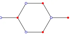
of P3⊕ {S1[1];S1[4]} is shown in Figure7.
The next theorem shows us a method for computing #(X) by breaking X into smaller disconnected configurations. A configuration [A, B] is connected if, given a∈A and b∈ B, there is a sequence {xk}mk=1 ∈ A∪B such that x1 = a, xm = b and xi is adjacent to xi+1
for each i [4]. In other words, there is a string in A∪B connecting a tob. A configuration is disconnected if it is not connected. The proof of Theorem 15 depends on the next result from the paper [4] (Theorem 6.1).
Theorem 14. Let [A, B] be a configuration and letr =h(A, B). If [X, Y] is a configuration withh(A, B) =h(X, Y), dE(a, y)> h(A, B)for alla∈A andy ∈Y, anddE(b, x)> h(A, B)
for all b∈B and x∈X, then #([A∪X, B∪Y]) = #([A, B])#([X, Y]).
In other words, if [U, V] is a disconnected configuration constructed from configurations [A, B] and [X, Y], with U =A∪X and V = B∪Y, then #([U, V]) = #([A, B])#([X, Y]). The next theorem describes another important computation technique.
Theorem 15. Let [A, B] and [X, Y] be finite configurations and let [U, V] = [A, B][a]⊕ [X, Y][y] for some a∈A and y∈Y. Then
#([U, V]) = #([A, B]) #([X, Y]) + #([A⊕S1[a], B]) #[X, Y ⊕S1[y]].
Proof. Without loss of generality, we assume h(A, B) = h(X, Y). Let s, t >0 with s+t =
h(A, B). LetC = (A)s∩(B)t be the largest element that lies betweenAandB at a distance
s from A, and let Z = (X)s∩(Y)t be the largest element that lies between X and Y at a
distancesfromX. Then in the configuration [U, V], the largest element betweenA∪X and
B ∪Y will be C ∪Z ∪ {c0}, where c0 is the point which lies between the newly adjacent
points a and y. See Figure 6 for an illustration.
We now consider which subsets Dof C∪Z∪ {c0}satisfy U DV. SinceD satisfiesU DV,
we know that [a′]D 6=∅, [b′]D 6=∅, [x′]D =6 ∅, and [y′]D 6=∅for all a′ ∈A, b′ ∈B, x′ ∈X, and
y′ ∈Y. We consider two cases.
Case 1 c0 6∈ D. In this case, let C′ = {d ∈ D : d ∈ [a′]D for somea′ ∈ A} and let Z′ =
D−C′. By construction, ifc′ ∈C′, thenc′ 6=c
0 and soc′ ∈C. ThusC′ ⊆C. Ifz′ ∈Z′,
then z′ 6=c0 and z′ ∈Z. Now, if a′ ∈ A and b′ ∈ B, we know [a′]D 6=∅ and [b′]D 6=∅.
Therefore, [a′]C′ 6=∅and [b′]C′ =6 ∅. SoC′ satisfiesAC′B. Similarly,Z′ satisfiesXZ′Y.
By Theorem14, the number of such sets D=C′∪Z′ is #([A, B]) #([X, Y]).
Case 2 c0 ∈D. In this case, we havec0 ∈[a]D and c0 ∈[y]D. The existence of the pointc0
inD allows for the potential removal of other points in D that are adjacent toa or y. In other words,D =C′∪ {c0} ∪Z′, whereC′ satisfiesAC′(B⊕S1[a]) and Z′ satisfies
(X⊕S1[y])Z′Y. The number of such setsD is #([A⊕S1[a], B])·#(X, Y ⊕S1[y]]).
Figure 8: P C3 2,3⊕S1.
As an example, consider the configuration X obtained by adjoining P3 and P2 as shown
in Figure 6. Theorem 15 shows
#(X) = #(P3) #(P2) + #(P3⊕S1) #(P2 ⊕S1).
Now Theorem 12 gives us #(P3 ⊕S1) = #(P3) + #(S5) = 18 + 3 = 21 and #(P2 ⊕S1) =
#(P2) + #(S3) = 7 + 1 = 8. So
#(X) = (18)(7) + (21)(8) = 294.
7
Finding
#(
P C
m,lk)
In this section, we determine a pair of recursive formulas to find #(P Ck
m,l). As the first step
in our computations, we determine #(X ⊕St) for t ≥ 2 for any finite configuration X in
terms of #(X) and #(X⊕S1).
Theorem 16. Let X be a finite configuration and t ≥2. Then
#(X⊕St) = Ft#(X⊕S1) +Ft−1#(X).
Proof. Using Theorem 12, we see that our theorem is certainly true with t = 2 and t = 3. We proceed by induction and suppose our theorem is true for all s, 1≤s≤t. Then
#(X⊕St+1) = #(X⊕St) + #(X⊕St−1)
= [Ft#(X⊕S1) +Ft−1#(X)] + [Ft−1#(X⊕S1) +Ft−2#(X)]
= (Ft+Ft−1)#(X⊕S1) + (Ft−1+Ft−2)#(X)
=Ft+1#(X⊕S1) +Ft#(X).
ByP Ck
m,l⊕Stwe mean the adjoin of St withP Cm,lk at a point antipodal to the connected
strings. An example of P C23,3 ⊕S1 is shown in Figure 8. A direct consequence of Theorem
16is
Corollary 17. For m≥2, k ≥1, l ≥1, and t≥2,
#(P Cm,lk ⊕St) =Ft#(P Cm,lk ⊕S1) +Ft−1#(P Cm,lk )
Now we add in the case when t= 1 for polygonal configurations. Note first that
Corollary 18. For m≥2 and t≥1,
#(Pm⊕St) =FtF2m+2+Ft−1L2m.
Proof. When t= 1, a direct application of Theorem 12gives us
#(Pm⊕S1) = #(Pm) + #(S2m−1) =L2m+F2m−2 =F2m+2 =F1F2m+2+F0L2m.
Fort ≥2, we use Theorem16 to obtain
#(Pm⊕St) =Ft#(Pm⊕S1) +Ft−1#(Pm) =FtF2m+2+Ft−1L2m.
We need one more preliminary calculation before we determine #(P Ck m,l).
Lemma 19. For m ≥2,
#(Pm⊕ {S1[1];S1[m+ 1]}) =Fm2+2.
Proof. Figure 7 shows an example of the configurations in question. By Theorem 12 and Corollary18,
#(Pm⊕ {S1[1];S1[m+ 1]}) = #(Pm⊕S1) + #(S2m−1⊕S1[m])
=F2m+2+ #(S2m−1) + #(Sm−1)2 =F2m+2+F2m−2+Fm2−2.
We use the identity
F2m =Fm2+1−Fm2−1
for m≥1 (see [7], Corollary 5.4 or [3], Identity 14 (note that fm =Fm+1)) to obtain
F2m+2+F2m−2+Fm2−2 =F2(m+1)+F2(m−1)+Fm2−2
= Fm2+2−Fm2+ Fm2 −Fm2−2+Fm2−2
=Fm2+2.
Now we derive recursive formulas for #(P Ck
m,l) and #(P Cm,lk ⊕S1) in terms of #(P Cm,lk−1)
and #(P Cm,lk−1 ⊕S1). Remember that #(P Cm,l1 ) = #(Pm) = L2m and #(P Cm,l1 ⊕S1) =
#(Pm⊕S1) = F2m+2. To include all cases together, we extend the Fibonacci sequence in
the negative direction by defining F−1 = 1. We also define X⊕S0 to be X for any finite
configurationX.
Theorem 20. For m ≥2, k ≥2, and l ≥1,
#(P Cm,lk ) = (L2mFl−2 +F2m+2Fl−1) #(P Cm,lk−1) + (L2mFl−1+F2m+2Fl) #(P C k−1
m,l ⊕S1)
where
#(P Cm,lk ⊕S1) = F2m+2Fl−2+Fl−1Fm2+2
#(P Cm,lk−1) + F2m+2Fl−1+FlFm2+2
* *
Figure 9: Using Theorem15to compute #(P Ck
m,l) and #(P C k m,l⊕S1).
Proof. We use Theorem 15 applied at the adjacent points indicated with an asterisk as illustrated in Figure 9, and Corollary 17:
#(P Cm,lk ) = #(Pm)#(P Cm,lk−1⊕Sl−1) + #(Pm⊕S1)#(P Cm,lk−1⊕Sl)
=L2m Fl−1#(P Cm,lk−1⊕S1) +Fl−2#(P Cm,lk−1)
+F2m+2 Fl#(P Cm,lk−1⊕S1) +Fl−1#(P Cm,lk−1)
= (L2mFl−1+F2m+2Fl) #(P Cm,lk−1 ⊕S1) + (L2mFl−2+F2m+2Fl−1) #(P Cm,lk−1).
Finally, we determine the recursive formula for #(P Ck
m,l ⊕S1) by using Theorem 15,
applied at the adjacent points indicated with an asterisk in Figure9. This gives us #(P Cm,lk ⊕S1) = #(P Cm,lk−1⊕Sl−1)#(Pm⊕S1) + #(P C
k−1
m,l ⊕Sl)#(Pm⊕ {S1[1];S1[m+ 1]}).
Therefore, Lemma 19and Corollary 17yield
#(P Cm,lk ⊕S1) = F2m+2#(P Cm,lk−1⊕Sl−1) + #(P Cm,lk−1⊕Sl)Fm2+2
=F2m+2 Fl−1#(P Cm,lk−1⊕S1) +Fl−2#(P Cm,lk−1)
+ Fl#(P Cm,lk−1⊕S1) +Fl−1#(P Cm,lk−1)
Fm2+2
= F2m+2Fl−1+FlFm2+2
#(P Cm,lk−1⊕S1)
+ F2m+2Fl−2+Fl−1Fm2+2
#(P Cm,lk−1).
As examples of the use of Theorem20,
#(P C32,1) =L6#(P C31,1) +F8#(P C31,1⊕S1)
= 18#(P3) + 21#(P3⊕S1)
= 18(18) + 21(21) = 765,
#(P C22,2) = F2m+2#(P Cm,lk−1) + [L2m+F2m+2] #(P Cm,lk−1 ⊕S1)
= 8#(P2) + [7 + 8]#(P2 ⊕S1)
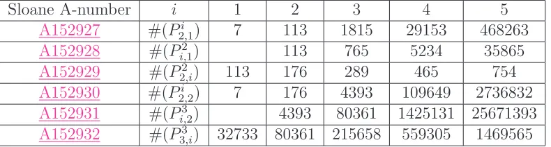
Sloane A-number i 1 2 3 4 5
A152927 #(Pi
2,1) 7 113 1815 29153 468263
A152928 #(Pi,21) 113 765 5234 35865
A152929 #(P2
2,i) 113 176 289 465 754
A152930 #(Pi
2,2) 7 176 4393 109649 2736832
A152931 #(P3
i,2) 4393 80361 1425131 25671393
[image:12.612.116.511.36.142.2]A152932 #(P33,i) 32733 80361 215658 559305 1469565
Table 1: Some polygonal chain sequences
and
#(P C22,3) = [L4F1+F6F2] #(P C21,3) + [L4F2+F6Fl] #(P C21,3⊕S1)
= [(7)(1) + (8)(1)]#(P2) + [(7)(1) + (8)(2)]#(P2⊕S1)
= (15)(7) + (23)(8) = 289.
8
Polygonal Chain Sequences
Theorem 20 gives us recursive formulas for finding #(P Ck
m,l). By fixing any two of m, k,
or l and letting the other parameter vary, we create infinite families of integer sequences. Examples of the first few terms of several of these sequences are given in Table1. We suspect that it is possible to define many new types of configurations in this geometry that provide more interesting and previously unknown integer sequences.
9
Asymptotic Behavior
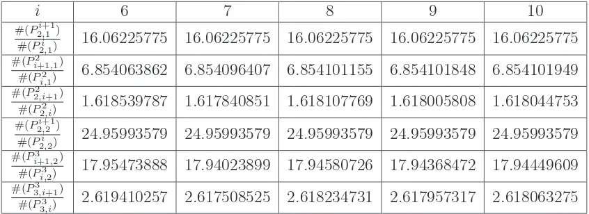
Polygonal chain sequences appear to exhibit asymptotically exponential behavior as the sequences of successive quotients in Table2illustrate. These sequences are natural extensions of string and polygonal sequences, both of which involve Fibonacci and Lucas numbers, so we might expect the ratios of polygonal chain sequences to do so as well. To understand this behavior, we investigate these quotients.
9.1
Fixing
m
and
l
In this section we consider the asymptotic behavior of the sequences obtained by letting k
vary for fixed values of m and l. For easier notation, let Xk,m,l = #(P Cm,lk ) and Yk,m,l =
#(P Ck
m,l⊕S1). Theorem20 shows that
i 6 7 8 9 10
#(P2i+1,1 )
#(Pi
2,1) 16.06225775 16.06225775 16.06225775 16.06225775 16.06225775
#(P2
i+1,1)
#(P2
i,1) 6.854063862 6.854096407 6.854101155 6.854101848 6.854101949
#(P2 2,i+1)
#(P2
2,i) 1.618539787 1.617840851 1.618107769 1.618005808 1.618044753
#(P2i+1,2 )
#(Pi
2,2) 24.95993579 24.95993579 24.95993579 24.95993579 24.95993579
#(P3
i+1,2)
#(P3
i,2) 17.95473888 17.94023899 17.94580726 17.94368472 17.94449609
#(P3 3,i+1)
#(P3
[image:13.612.100.523.35.189.2]3,i) 2.619410257 2.617508525 2.618234731 2.617957317 2.618063275
Table 2: Ratios of polygonal chain sequences to 8 decimal places.
for values of am,l, bm,l, cm,l, and dm,l that depend on only m and l. We can determine the
asymptotic behavior of Xk,m,l by writing this system in matrix form:
Xk,m,l Yk,m,l =
am,l bm,l
cm,l dm,l
Xk−1,m,l
Yk−1,m,l
.
LetMm,l =
am,l bm,l
cm,l dm,l
. Then Xk,m,l Yk,m,l
= (Mm,l) k−1
X1,m,l
Y1,m,l
.
The eigenvalues of Mm,l are
λm,l =
(dm,l+am,l) +
p
(dm,l−am,l)2+ 4bm,lcm,l
2
and
λm,l=
(dm,l+am,l)−
p
(dm,l−am,l)2+ 4bm,lcm,l
2 .
Since (dm,l−am,l)2+ 4bm,lcm,l >0, we see that Mm,l has two distinct real eigenvalues. Thus
Mm,lis diagonalizable to the matrixDm,l =
λm,l 0
0 λm,l
. IfQm,lis the matrix whose columns
are the eigenvectors ofMm,l, then
Xk,m,l
Yk,m,l
= Qm,l
"
(λm,l)k−1 0
0 λm,l
k−1 #
Q−m,l1 !
X1,m,l
Y1,m,l
.
Note thatQm,l =
"
1 1
λm,l−am,l
bm,l
dm,l−λm,l
bm,l
#
and Q−m,l1 = 1
2λm,l−(am,l+dm,l)
λ
m,l−dm,l bm,l
λm,l−am,l −bm,l
Since X1,m,l =L2m and Y1,m,l =F2m+2, we have
Xk,m,l =Rm,lλkm,l−1+Sm,lλ k−1
m,l (2)
where Rm,l=
1
2λm,l−(am,l+dm,l)
((λm,l−dm,l)L2m+bm,lF2m+2) and
Sm,l =
1
2λm,l−(am,l+dm,l)
((λm,l−am,l)L2m−bm,lF2m+2). So (2) provides a non-recursive
formula for computing Xk,m,l. Now λm,l > λm,l, so we have
Xk,m,l
Xk−1,m,l
= Rm,lλ
k−1
m,l +Sm,lλ k−1
m,l
Rm,lλkm,l−2+Sm,lλ k−2
m,l
=
Rm,lλm,l+Sm,lλm,l
λ
m,l
λm,l
k−2
Rm,l+Sm,l
λ
m,l
λm,l
k−2
→ Rm,lRλm,l
m,l
=λm,l
ask → ∞. Thus,
lim
k→∞
Xk,m,l
Xk−1,m,l
=λm,l.
The values of am,l, bm,l, cm,l, and dm,l are given by Theorem 20:
am,l=L2mFl−2+F2m+2Fl−1, bm,l =L2mFl−1+F2m+2Fl,
cm,l=F2m+2Fl−2+Fl−1Fm2+2, and dm,l =F2m+2Fl−1 +FlFm2+2.
Thus the sequence of polygonal chain numbers as k varies for fixed m and l behaves asymptotically as the exponential sequence with ratio λm,l. For example, λ2,1 = 8 +
√ 65≈ 16.06225775 andλ2,2 = 25+3
√
69
2 ≈24.95993579 (compare to the ratios in Table 2).
9.2
Limits of Fibonacci and Lucas Sequences
To determine the asymptotic behavior of the sequences{Xk,m,l}as eithermorlvary, we will
need some limits of sequences of quotients of Fibonacci and Lucas numbers. Let ϕ = 1+2√5 be the golden ratio. The following results concerning Fibonacci and Lucas numbers are well known.
• lim
m→∞
Fm+1
Fm
=ϕ ([7] Corollary 8.5, [8] (25))
• lim
m→∞
Lm+1
Lm
=ϕ ([7] Corollary 8.7, [8] (25))
• ϕm =F
• lim
m→∞
Fm+j
Fm
=ϕj forj ≥0 ([3] Corollary 31, [8] (27))
• Forj ≥0, lim
m→∞
Lm+j
Lm
=ϕj ([8] (27))
We will also need other limits of ratios of Fibonacci and Lucas numbers.
Lemma 21. For m ≥2 and j ≥0,
1. Forj ≥0, lim
m→∞
Lm
Fm+j
= 1 +ϕ
2
ϕj+1
2. lim
m→∞
F2m+2
F2
m+2
= ϕ
4−1
ϕ4 =
1 +ϕ2 ϕ3
3. lim
m→∞
F2m+2
Fm2+3
= ϕ
4−1
ϕ6 =
1 +ϕ2
ϕ5
4. lim
m→∞
F2m+4
F2
m+2
= ϕ
4−1
ϕ2 =
1 +ϕ2 ϕ
5. lim
m→∞
L2m
F2
m+2
= (ϕ
2+ 1)2
ϕ6
Proof. We prove 2 and 5, the remainder are similar. Recalling that ϕ2−1 = ϕ,
lim
m→∞
F2m+2
Fm2+2
= lim
m→∞
Fm2+2−Fm2
Fm2+2
= lim
m→∞1−
Fm
Fm+2
2
= 1−
1
ϕ2
2
= ϕ
4−1
ϕ4
= (1 +ϕ
2)ϕ
ϕ4
= 1 +ϕ
2
Finally, we use Identity 13 from the book [3] (F2m+1 =Fm2 +Fm2+1) to see
lim
m→∞
L2m
F2
m+2
= lim
m→∞
F2m−1+F2m+1
F2
m+2
= lim
m→∞ (F2
m−1+Fm2) + (Fm2 +Fm2+1)
F2
m+2
= lim
m→∞
Fm−1
Fm+2
2
+ 2
Fm
Fm+2
2
+
Fm+1
Fm+2
2 = 1 ϕ3 2 + 2 1 ϕ2 2 + 1 ϕ 2
= 1 + 2ϕ
2+ϕ4
ϕ6
= (ϕ
2+ 1)2
ϕ6 .
9.3
Fixing
k
and
l
In this section, we fixk and l and let m vary and investigate the asymptotic behavior of the resulting sequence Xk,m,l. We will need to know limits of ratios of the terms am,l, bm,l, cm,l
and dm,l as m approaches infinity.
Lemma 22. Let Gl= (
1+ϕ2)F
l−1+ϕ3Fl
(1+ϕ2)F
l−2+ϕ3Fl−1. Then for l≥1,
1. lim
m→∞
am+1,l
am,l
=ϕ2
2. lim
m→∞
bm+1,l
am,l
=ϕ2Gl
3. lim
m→∞
bm,l
am,l
=Gl
4. lim m→∞ cm,l am,l = ϕ 3
1 +ϕ2
5. lim
m→∞
cm+1,l
am,l
= ϕ
5
1 +ϕ2
6. lim m→∞ dm,l am,l = ϕ3
1 +ϕ2
Gl.
7. lim
m→∞
dm+1,l
am,l
=
ϕ5
1 +ϕ2
Proof. We prove 5, the others are similar:
lim
m→∞
cm+1,l
am,l
= lim
m→∞
F2m+4Fl−2 +Fm2+3Fl−1
L2mFl−2 +F2m+2Fl−1
= lim
m→∞
F2m+4
F2m+2
Fl−2 +
F2
m+3
F2m+2
Fl−1
L2m
F2m+2
Fl−2+Fl−1
= (
ϕ2)F
l−2+
ϕ5
ϕ2+1
Fl−1
1+ϕ2
ϕ3
Fl−2+Fl−1
=
ϕ5
1 +ϕ2
1+ϕ2
ϕ3
Fl−2+Fl−1
1+ϕ2
ϕ3
Fl−2+Fl−1
= ϕ
5
1 +ϕ2.
Before we can analyze the asymptotic behavior of the polygonal chain sequence, we need to understand how the sequences {Yk,m,l}and {Xk,m,l} are related asm varies.
Lemma 23. For k ≥1,
lim m→∞ Yk,m,l Xk,m,l = ϕ 3
1 +ϕ2.
Proof. When k = 1 we have lim
m→∞
Y1,m,l
X1,m,l
= lim
m→∞
F2m+2
L2m
= 1 1
ϕ3 + 1ϕ
= ϕ
3
1 +ϕ2. So the claim is
true fork= 1. We proceed by induction and assume the claim is true for some k ≥1. Then (1) shows
lim
m→∞
Yk+1,m,l
Xk+1,m,l
= lim
m→∞
cm,lXk,m,l+dm,lYk,m,l
am,lXk,m,l+bm,lYk,m,l
= lim m→∞ c m,l am,l
+dm,l
am,l
Yk,m,l
Xk,m,l
1 +bm,l
am,l Yk,m,l Xk,m,l = ϕ3
1+ϕ2
+1+ϕ3ϕ2
Gl
ϕ3
1+ϕ2
1 +Gl
ϕ3
ϕ2+1
= ϕ
3
Now we can identify the asymptotic behavior of the polygonal chain sequence when m
varies.
Theorem 24. For k ≥1 and l ≥1,
lim
m→∞
Xk,m+1,l
Xk,m,l
=ϕ2k and lim
m→∞
Yk,m+1,l
Xk,m,l
= ϕ
2k+3
1 +ϕ2.
Proof. The proof will be by induction on k. Now X1,m,l = L2m and lim m→∞
X1,m+1,l
X1,m,l
=
lim
m→∞
L2m+2
L2m
= ϕ2. Also, Y1,m,l = F2m+2 and lim
m→∞
Y1,m+1,l
X1,m,l
= lim
m→∞
F2m+4
L2m
= 1 1
ϕ5 +
1
ϕ3 =
ϕ5
1 +ϕ2. Thus, our theorem is true when k= 1. Assume the theorem is true for somek ≥1.
Then
lim
m→∞
Xk+1,m+1,l
Xk+1,m,l
= lim
m→∞
am+1,lXk,m+1,l+bm+1,lYk,m+1,l
am,lXk,m,l+bm,lYk,m,l
= lim
m→∞
a
m+1,l
am,1
Xk,m+1,l
Xk,m,l
+bm+1,l
am,l
Yk,m+1,l
Xk,m,l
1 +bm,l
am,1
Yk,m,l
Xk,m,l
=
(ϕ2) ϕ2k
+ (ϕ2G
l)
ϕ2k+3
1+ϕ2
1 + (Gl)
ϕ3
1+ϕ2
=ϕ2k+2
and
lim
m→∞
Yk+1,m+1,l
Xk+1,m,l
= lim
m→∞
cm+1,lXk,m+1,l+dm+1,lYk,m+1,l
am,lXk,m,l+bm,lYk,m,l
= lim
m→∞
c
m+1,l
am,l
Xk,m+1,l
Xk,m,l
+dm+1,l
am,l
Yk,m+1,l
Xk,m,l
1 +bm,l
am,l Yk,m,l Xk,m,l = ϕ5
1+ϕ2
ϕ2k
+1+ϕ5ϕ2
Gl
ϕ2k+3
1+ϕ2
1 + (Gl)
ϕ3
1+ϕ2
= ϕ
2k+5
1 +ϕ2.
So the sequence of polygonal chain numbers asm varies for fixedk andl behaves asymp-totically as the exponential sequence with ratio ϕ2k. For example, ϕ4 ≈ 6.854101954 and
9.4
Fixing
k
and
m
In this section, we fixk and m and letl vary and investigate the asymptotic behavior of the resulting sequenceXk,m,l. Again, we begin with limits of sequences of ratios ofam,l, bm,l, cm,l,
and dm,l, this time asl goes to infinity.
Lemma 25. Let Hm =
F2m+2+Fm2+2ϕ
L2m+F2m+2ϕ . Then for m ≥2,
1. lim
l→∞
am,l+1
am,l
=ϕ
2. lim
l→∞
bm,l
am,l
=ϕ
3. lim
l→∞
bm,l+1
am,l
=ϕ2
4. lim
l→∞
cm,l
am,l
=Hm
5. lim
l→∞
cm,l+1
am,l
= (ϕ)Hm
6. lim
l→∞
dm,l+1
am,l
= ϕ2 Hm.
Proof. We verify 5 and leave the others for the reader:
lim
l→∞
cm,l+1
am,l
= lim
l→∞
F2m+2Fl−1+Fm2+2Fl
L2mFl−2+F2m+2Fl−1
= lim
l→∞
F2m+2+Fm2+2
Fl
Fl−1
L2m
F
l−2
Fl−1
+F2m+2
= F2m+2+F
2
m+2ϕ
L2m
1
ϕ
+F2m+2
= (ϕ)
F2m+2+Fm2+2ϕ
L2m+F2m+2ϕ
.
Now we need to understand the relationship between the sequence {Yk,m,l} and the
se-quence {Xk,m,l} as l goes to infinity.
Lemma 26. For k ≥2, m ≥2,
lim
l→∞
Yk,m,l
Xk,m,l
Proof. When k = 2 we have
lim
l→∞
Y2,m,l
X2,m,l
= lim
l→∞
cm,lX1,m,l+dm,lY1,m,l
am,lX1,m,l+bm,lY1,m,l
= lim l→∞ c m,l am,l
X1,m,l+
d
m,l
am,l
Y1,m,l
X1,m,l+
b
m,l
am,l
Y1,m,l
= (Hm)L2m+ (ϕHm)F2m+2
L2m+ϕF2m+2
=Hm.
So the lemma is true for k = 2. We proceed by induction and assume the lemma is true for some k≥2. Then (1) shows
lim
l→∞
Yk+1,m,l+1
Xk+1,m,l+1
= lim
l→∞
cm,lXk,m,l+dm,lYk,m,l
am,lXk,m,l+bm,lYk,m,l
= lim l→∞ c m,l am,l
+dm,l
am,l
Yk,m,l
Xk,m,l
1 +bm,l
am,l
Yk,m,l
Xk,m,l
= (Hm) + (ϕHm) (Hm) 1 + (ϕ) (Hm)
=Hm.
Now we determine the asymptotic behavior of the polygonal chain sequences if we allow
l to vary.
Theorem 27. For k ≥2 and m≥2,
lim
l→∞
Xk,m,l+1
Xk,m,l
=ϕk−1 and lim
l→∞
Yk,m,l+1
Xk,m,l
=ϕk−1(Hm).
Proof. The proof will be by induction on k. Recall that X1,m,l = L2m and Y1,m,l = F2m+2
We first verify thek = 2 case. Equation (1) shows
lim
l→∞
X2,m,l+1
X2,m,l
= lim
l→∞
am,l+1X1,m,l+1+bm,l+1Y1,m,l+1
am,lX1,m,l+bm,lY1,m,l
= lim l→∞ a m,l+1 am,l
X1,m,l+1+
b
m,l+1
am,l
Y1,m,l+1
X1,m,l+
b
m,l
am,l
Y1,m,l
= ϕL2m+ϕ
2F 2m+2
L2m+ϕF2m+2
and
lim
l→∞
Y2,m,l+1
X2,m,l
= lim
l→∞
cm,l+1X1,m,l+1+dm,l+1Y1,m,l+1
am,lX1,m,l+bm,lY1,m,l
= lim l→∞ c m,l+1 am,l
X1,m,l+1+
d
m,l+1
am,l
Y1,m,l+1
X1,m,l+
b
m,l
am,l
Y1,m,l
= (ϕ) (Hm)L2m+ (ϕ
2H
m)F2m+2
L2m+ϕF2m+2
=ϕHm.
Now the general cases:
lim
l→∞
Xk+1,m,l+1
Xk+1,m,l
= lim
l→∞
am,l+1Xk,m,l+1+bm,l+1Yk,m,l+1
am,lXk,m,l+bm,lYk,m,l
= lim
l→∞
a
m,l+1
am,l
Xk,m,l+1
Xk,m,l
+bm,l+1
am,l
Yk,m,l+1
Xk,m,l
1 +bm,l
am,l
Yk,m,l
Xk,m,l
= (ϕ) ϕ
k−1
+ (ϕ2) ϕk−1H
m
1 + (ϕ) (Hm)
=ϕk
and
lim
l→∞
Yk+1,m,l+1
Xk+1,m,l
= lim
l→∞
cm,l+1Xk,m,l+1+dm,l+1Yk,m,l+1
am,lXk,m,l+bm,lYk,m,l
= lim
l→∞
c
m,l+1
am,l
Xk,m,l+1
Xk,m,l
+dm,l+1
am,l
Yk,m,l+1
Xk,m,l
1 +bm,l
am,l
Yk,m,l
Xk,m,l
= (ϕHm) ϕ
k−1
+ (ϕ2Hm) ϕk−1Hm
1 + (ϕ) (Hm)
=ϕkHm.
So the sequence of polygonal chain numbers asl varies for fixedk andm behaves asymp-totically as the exponential sequence with ratio ϕk−1. For example, ϕ ≈ 1.618033988 and
10
Conclusion
The asymptotic growth rates of polygonal chain sequences are functions of the golden ratio
ϕ. Since polygonal chains are constructed from string and polygonal configurations and lim
l→∞
#(Sl+1)
#(Sl)
= ϕ and lim
m→∞
#(Pm+1)
#(Pm)
= ϕ2, this should not be surprising in hindsight.
That the asymptotic ratios of the polygonal chain sequences have such nice closed forms is, however, somewhat surprising given the complex nature of betweenness in this geometry.
Polygonal chain sequences provide a three parameter family of integer sequences previ-ously unidentified in The On-Line Encyclopedia of Integer Sequences [10]. These sequences have interesting geometric interpretations as the number of compact sets at each location between the component sets that make up the polygonal chain. We suspect that there are many other similar families of unknown sequences just waiting to be found.
11
Acknowledgements
This work was supported by National Science Foundation grant DMS-0451254. The authors also thank Grand Valley State University for hosting and supporting a Research Experiences for Undergraduates program.
References
[1] M. Barnsley, Fractals Everywhere, Second Edition, Academic Press Professional, 1998.
[2] C. Bay, A. Lembcke, and S. Schlicker, When lines go bad in hyperspace, Demonstratio Math., 38 (2005), 689–701.
[3] A. T. Benjamin and J. J. Quinn, Proofs That Really Count, Mathematical Association of America, 2003.
[4] C. Blackburn, K. Lund, S. Schlicker, P. Sigmon, and A. Zupan, A missing prime config-uration in the Hausdorff metric geometry, to appear,J. Geom.
[5] L. M. Blumenthal, Theory and Applications of Distance Geometry, Oxford University Press, 1953.
[6] D. Braun, J. Mayberry, A. Powers, and S. Schlicker, A singular introduction to the Hausdorff metric geometry, Pi Mu Epsilon J., 12 No. 3, (2005), 129–138.
[7] T. Koshy, Fibonacci and Luca Numbers with Applications, John Wiley & Sons, 2001.
[8] E. Lucas, Th´eorie des fonctions num´eriques simplement p´eriodiques, Amer. J. Math. 1 (1878), 184–240, 289–321.
[9] K. Lund, P. Sigmon, and S. Schlicker, Fibonacci sequences in the space of compact sets,
[10] N. J. A. Sloane, (2007), The On-Line Encyclopedia of Integer Sequences, published electronically at http://www.research.att.com/~njas/sequences/
2000 Mathematics Subject Classification: Primary 51F99; Secondary 11B83.
Keywords: Hausdorff metric, configuration, metric geometry, polygonal chains, Fibonacci numbers, Lucas numbers.
(Concerned with sequencesA000032,A000045,A152927,A152928,A152929,A152930,A152931, and A152932.)
Received August 22 2008; revised version received December 22 2008. Published in Journal of Integer Sequences, December 22 2008.