www.elsevier.nlrlocatereconbase
Revisiting Rogowski and Newhouse on the
indirect costs of teaching: a note on functional
form and retransformation in Medicare’s
payment formulas
Kathleen Dalton
a,), Edward C. Norton
ba
Cecil G. Sheps Center for Health SerÕices Research, CBa7590 725 Airport Road, Chapel Hill,
NC 27599-7590, USA
b
Department of Health Policy and Administration School of Public Health UniÕersity of North
Carolina at Chapel Hill, Chapel Hill, NC, USA
Received 1 November 1999; received in revised form 1 May 2000; accepted 26 May 2000
Abstract
In 1992 Rogowski and Newhouse identified errors in functional form and retransforma-tion in the econometric model that underlies Medicare’s payments to teaching hospitals. We re-estimate their model and expand on their work, with data from the following decade. We
Ž .
find: 1 the functional form imposed by Health Care Financing Administration’s original
Ž .
specification of the teaching variable is supported by the data; 2 there is no evidence of a
Ž .
threshold effect when the teaching intensity variable is appropriately specified; 3 there is no longer evidence of heteroscedasticity across teaching hospital types, consequently there is no need to incorporate re-transformation factors into the payment formula. We attribute the differences in our findings to secular changes in the hospital industry and improvements in variable measurement.q2000 Elsevier Science B.V. All rights reserved.
Ž .
Keywords: Hospital costs; Teaching hospitals; Prospective payment system PPS ; Retransformation
)Corresponding author. Tel.:q1-919-966-7957; fax:q1-919-966-5764.
Ž .
E-mail address: kathleen [email protected] K. Dalton .–
0167-6296r00r$ - see front matterq2000 Elsevier Science B.V. All rights reserved.
Ž .
1. Introduction
In 1992 Rogowski and Newhouse published a comprehensive assessment of the
Ž .
regression model developed by the Health Care Financing Administrations HCFA , that serves as the basis for Medicare’s current system of payment adjustments to
Ž
hospitals participating in graduate medical education Rogowski and Newhouse,
.
1992 . The purpose of this note is to determine if their findings still apply to cost data collected over 10 years later, after a period of substantial structural change in the hospital industry. This is an appropriate time to review earlier work, because the Medicare Payment Advisory Commission is currently reviewing the empirical evidence and policy implications behind Medicare’s medical education
adjust-Ž .
ments in order to recommend changes to Congress MedPAC, 1999 . The indirect
Ž .
medical education IME formulas governing these payments affect the distribu-tion of nearly US$5 billion of US$78 billion now paid to short-stay hospitals, and they are sensitive for political as well as budgetary reasons. Over time, IME payments have acquired a policy justification in addition to their empirical basis, in that the adjustment has intentionally been allowed to exceed estimated cost differentials in order to fulfill a policy objective of directing more Medicare funds to teaching hospitals. Resolution of the specification issues in the empirical model remains important, however, in order to identify how much of the payment adjustment reflects true product differentiation and how much should be viewed as an educational subsidy.
1.1. Background
HCFA’s original hospital cost model as described by Pettengill and Vertrees
Ž1982 and Lave 1985 , was a log-linear specification where the logarithm of. Ž .
Medicare operating cost per case was estimated as a function of teaching intensity, with controls for case mix, hospital size, regional wage variation and metropolitan area size. The analysis was conducted on hospital-level arithmetic means, using accounting data from federal fiscal year 1981. The ordinary least squares estima-tion was run with no second-order terms, imposing an assumpestima-tion of a diminishing marginal effect of changes in teaching intensity on unit cost, with a single teaching coefficient computed across the full sample of hospitals.
Although the specific formula has changed over time, coefficients from this regression have been used to adjust the prices paid by Medicare to teaching
Ž .
hospitals since the start of the Prospective Payment System PPS . In the enabling
Ž .
restricted the control variables and their parameters to conform to the PPS payment formula. The teaching coefficient from this restricted version was adopted as part of PL 99-272 in 1985, and has remained in effect ever since. For reasons related to policy concerns rather than empirical evidence, the teaching adjustment has also been deliberately increased to levels in excess of the measured cost
Ž
differential, by applying a multiplier to the adjustment that has ranged from 2.0 in
. Ž
the 1982 legislation to 1.35 mandated for 2002, by the Balanced Budget
.
Refinement Act of 1999 .
After its initial introduction into legislation, HCFA’s model was the subject of a
Ž
moderate amount of attention in the health economics literature Anderson and
.
Lave 1986; Welch 1987; Thorpe 1988; Sheingold 1990 . The econometric analysis was criticized primarily for bias attributable to omitted location variables and other operating characteristics, for the theoretical inconsistency of including hospital size in the estimation while failing to include it in the payment formulas, and for failure to recognize a difference in the strength of the teaching effect between large and small teaching programs. Thorpe also speculated that HCFA’s
specifica-Ž
tion of the teaching variable as the log of one plus the ratio of residents to staffed
.
beds introduced additional bias into the estimation insofar as the true relationship is assumed to be between cost per case and the ratio itself, without the constant.
Ž .
Rogowski and Newhouse 1992 systematically assessed these and additional problems in HCFA’s original model, using data from discharges in federal fiscal year 1984. They conducted regression diagnostics to assess heteroscedasticity and
Ž
omitted variable bias, specified an alternative teaching variable computed as the
.
natural log of the sum of the resident-to-bed ratio plus 0.0001 and generalized the log-linear assumption by constructing spline functions on their revised teaching variable to allow for multiple slope coefficients. They addressed additional
Ž
technical shortcomings of the model by adding weights to account for estimation
.
Rogowski and Newhouse closed, however, with a caution against revising the payment formula until further research could incorporate the effects of a new
Ž
payment adjustment for hospitals with high indigent care loads the
disproportion-.
ate share, or DSH, adjustment, implemented in 1985 and until the stability of their results could be examined over time. It is in that spirit that we offer the following update to their findings.
2. Data
We re-estimated hospital costs using models that are similar to HCFA’s original model and to those developed by Rogowski and Newhouse, using 2 years of data from cost reports filed for the federal fiscal years 1994 and 1995. Costs are analyzed for all short-stay facilities paid under PPS, with at least 50 Medicare discharges. Quarterly moving averages of the PPS Input Price Index were used to deflate mean operating costs per discharge. Medicare’s Case-Mix Index Files and Wage Index Files provided control variables for case severity and regional
Ž .
variation in factor prices. The ratio of interns and residents to beds IRB for each teaching hospital was derived from the indirect medical education payments reported on the settlement pages of the cost reports. A total of 4988 hospitals contributed 9627 observations to the final estimation sample, which is summarized in Table 1.
Table 1
Sample description
a
All hospitals Non-teaching Teaching
Number of observations 9627 7475 2152
Number of unique hospitals 4988 3903 1145
Ž .
Average real operating cost per day 1987 dollars US$3553 US$3163 US$4907
Average case mix index 1.2490 1.1849 1.4714
Intern and resident-to-staffed bed ratio: mean 0.1823
Intern and resident-to-staffed bed ratio: median 0.0948
Ž .
Average number of staffed beds acute care only 148 105 297
Average wage index 0.9200 0.8873 1.0336
% Located in non-MSA 44% 55% 6%
Ž .
% Located in small MSA population-1 million 26% 23% 37%
Ž .
% Located in large MSA population)1 million 30% 22% 57%
% Receiving DSH payments 40% 33% 65%
Ž .
Mean Medicaid utilization % days 13% 12% 17%
a
3. Methods
3.1. Variable specification
We retained the specification of the dependent variable as the natural log of the average operating cost per case. We developed four variations on the original cost model, each derived from a different formulation of the variable measuring teaching intensity. The first model minimizes parametric assumptions by specify-ing teachspecify-ing intensity as a set of dummy variables constructed by level of the IRB ratio, using intervals of 0.07 in the value of the ratio from 0 to 0.70, and a single group for hospitals with ratios above 0.70. This results in 11 dummy variables, with the non-teaching group serving as a reference. Our purpose in presenting these semi-parametric results is to provide a basis for comparison against which we can assess the restrictions in functional form that are imposed by each of our continuous variable models. Considering the policy application of the model, a parametric specification is preferred to a specification with indicator variables — if the parametric model fits the data well — because indicator variables would introduce notches into the payment formula.
The remaining models are derived from continuous specifications of teaching intensity including:
1. the actual value of the IRB, which ranges from zero to 1.3 2. the natural log of the IRB after adding a constant of 1.0 3. the natural log of the IRB after adding a constant of 0.001.
Because the dependent variable is logged, the second specification imposes an exponential form on the model similar to one used by HCFA in 1990 to estimate
Ž .
the IME adjustment for the PPS capital cost payment Phillips, 1992 . The third specification is the same as HCFA’s original measure of teaching intensity, and the fourth is similar to Rogowski and Newhouse’s recommended alternative. In keeping with Rogowski and Newhouse, we also explored generalizations of each of the continuous forms, using spline functions to identify significant thresholds for differences in the slope coefficient on teaching.
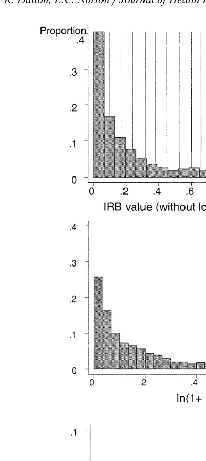
Distributions of the non-zero values of each of our teaching variables are presented in Fig. 1. Four-fifths of short stay hospitals do not participate in graduate medical education. Among those that do, the distribution of the resident-to-bed ratio is still highly skewed, with the majority of teaching hospitals showing ratios that are less than 0.10. Using a log transformation with a constant smaller than 1.0 reduces the skewness, but it also increases the influence of these smaller programs in the estimation.
3.2. Estimation
Ž
Fig. 1. Comparing distributions of the teaching variable across alternative specifications note:
.
distributions exclude observations for non-teaching hospitals .
Ž
capture any fixed cost differentials associated with minor teaching status 0-IRB
. Ž .
-0.30 or major teaching status IRBG0.30 . Neither the teaching intensity measures nor the indicator variables by teaching status estimate the economic costs of teaching per se. They serve, rather, as proxy measures for cost differen-tials from unobserved characteristics of care delivered in teaching settings. The empirical component of the IME adjustment can be viewed as a price premium that is predicated on the assumption that these estimates reflect legitimate product differentiation. For each specification of the teaching variable, the equation is:
ln operating cost
Ž
rcase.
saqbteaching intensityqg1ln CMIŽ
.
qg2ln wage index
Ž
.
qg3 lnŽ
abeds.
qg4small urban statusqg5large urban status
qg6 yearq´
Ž .
1whereb is the vector of predictors on the set of teaching variables appropriate to each model, including the fixed teaching effects measured by the major or minor teaching status indicators, where applicable. Weighted least squares estimation was applied using analytic weights derived from the number of discharges contributing to each hospital mean, with Huber–White robust standard errors with clustering by hospital.
Without interaction or other second-order terms in the equations, all but the first of our specifications impose an assumption that the marginal effect of teaching on the logged dependent variable is linear and constant across the estimation sample. To assess the reasonableness of this assumption, we plotted results from the models using continuous teaching variables against results com-puted from the dummy variable model. For formal tests of log-linearity, however, spline functions were constructed from each of the three continuous teaching
Ž .
variables models 2,3 and 4 to test for differences in the teaching slope coeffi-cients by ranges of IRB values. Spline knots were initially set at each variable’s equivalent to IRB ratios of 0.03, 0.15, 0.30 and 0.60. Because of the relatively small sub-group size the splines for highest two groups were collapsed into one. In Rogowski and Newhouse the teaching hospitals were initially divided into six equal groups to establish spline knots. The first five were later collapsed into one group, leaving one knot at 0.25 that isolated the top 17% of teaching facilities. Our upper knot is set higher because the ratios have increased over time; 20% of teaching hospitals in our sample had ratios above 0.30.
Rogowski and Newhouse found that their formulation of the teaching variable that uses a smaller constant and allows for multiple slope coefficients reduced the model’s susceptibility to bias from omitted variables. To test whether this was true in our data, all four of our models were repeated using a specification that eliminated the variable for number of hospital beds, and another that added a Medicaid utilization variable and two sets of dichotomous variables by census
Ž
.
to follow Rogowski and Newhouse’s expanded model as closely as possible. We present the resulting differences in estimated teaching effects to compare the omitted variable bias across each of the specifications.
3.3. Retransformation
To avoid confusion from the different units of measurement in teaching intensity, all results are expressed in terms of the expected teaching effect. This is defined as the percent difference in expected costs between teaching hospitals and
Ž .
non-teaching hospitals assuming similarity in all covariates other than teaching and can be expressed as:
Holding other covariates constant and assuming for now constant variance, the numerator and denominator terms for eXg
and e´
cancel out. In all but the
Ž .
ln 0.001qIRB specification, the denominator of the right-hand side equals one, and the expected teaching effects can be measured by eŽXb.
y1, where X represents the teaching variable as it is entered into the estimation of logged cost.
Ž .
In the case where teaching is specified as ln 0.001qIRB , however, the denomi-nator in the ratio of expected costs will always retain a term equal to elnŽ0q0.001.b,
Ž .b
or 0.001 .
Because Rogowski and Newhouse identified systematic differences in the distribution of the variance across teaching hospital subgroups, we could not assume that the exponentiated error terms in the above ratios would cancel out. We computed smearing estimates for the expected value of the re-transformed error computed from the mean of the exponentiated residuals, appropriate when
Ž .
the error is assumed to be non-normally distributed Duan, 1983; Manning, 1998 . Let s denote smearing estimates as computed across the residuals from the appropriate group of observations. The formulas for expected teaching cost differentials in our four models can be summarized as follows:
<
using a log-linear function, on 1
Ž
qIRB.
using a log-linear function, on 0.001
Ž
qIRB.
where bcat is the coefficient on the dummy variable and bstatus is the coefficient
Ž .
on the major or minor teaching status indicator, as appropriate. Eq. 3 includes an
Ž .
additional variance correction factor forbcat as recommended by Kennedy 1981 , but where the standard error of the dummy coefficient is small, this correction has only a very slight influence on the results.
If groupwise heteroscedasticity is not present in our data, the ratio of the two smearing estimates will approximate one. If the expected teaching effect is small, however, a factor very close to 1.0 can still have a large proportional effect on the model interpretation and the resulting payment adjustments. To establish the necessity of retaining the retransformation correction factors in the computations, we therefore subjected the exponentiated residuals to further tests to evaluate whether heteroscedasticity is systematic with respect to the size of the teaching program.
4. Results
4.1. Comparing estimated teaching cost differentials across specifications
Cost differentials computed from the dummy variable model increase steadily in strength from the first through the tenth category of teaching intensity. All groups but the first test significantly different from zero at a pF0.001 level, and
Ž .
in the first category IRBF0.07, mean value approximately 0.03 the parameter is
Ž .
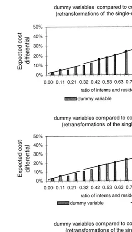
still marginally significant ps0.063 . Fig. 2 plots the estimated teaching cost differentials from each of the continuous specifications against those computed from the dummy variables on categories of teaching, where bars representing the expected teaching effect by IRB category are placed approximately at the mean value of the ratio within that category. Regression results are provided in Tables 2 and 3.
There are positive but insignificant fixed teaching effects in both the
exponen-Ž .
tial model and the log–log model based on 1qIRB . Within the range of ratios applicable to the great majority of teaching hospitals, expected teaching effects are very similar between the exponential form and the logarithmic form that uses a
Ž .
Ž
Fig. 2. Estimated teaching differentials under alternative specifications of teaching intensity note: bars
.
are placed approximately at the mean IRB value within each dummy variable category .
a ratio of 0.91, the cost differential predicted by the exponential function is 30.9%,
Ž .
()
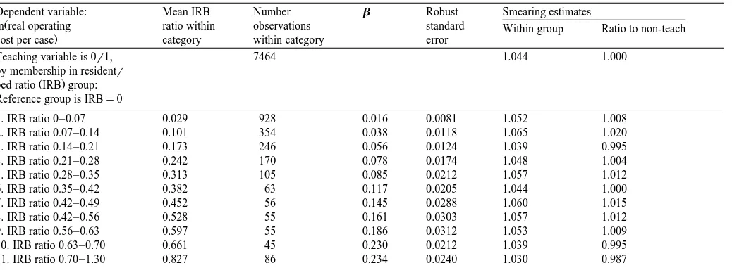
Results from regression using categorical teaching intensity variables — parameter estimates on teaching variables only
Dependent variable: Mean IRB Number b Robust Smearing estimates
Ž
ln real operating ratio within observations standard Within group Ratio to non-teach
.
cost per case category within category error
Teaching variable is 0r1, 7464 1.044 1.000
by membership in residentr
Ž .
bed ratio IRB group: Reference group is IRBs0
1. IRB ratio 0–0.07 0.029 928 0.016 0.0081 1.052 1.008
2. IRB ratio 0.07–0.14 0.101 354 0.038 0.0118 1.065 1.020
3. IRB ratio 0.14–0.21 0.173 246 0.056 0.0124 1.039 0.995
4. IRB ratio 0.21–0.28 0.242 170 0.078 0.0174 1.048 1.004
5. IRB ratio 0.28–0.35 0.313 105 0.085 0.0212 1.057 1.012
6. IRB ratio 0.35–0.42 0.382 63 0.117 0.0205 1.044 1.000
7. IRB ratio 0.42–0.49 0.452 56 0.145 0.0288 1.060 1.015
8. IRB ratio 0.42–0.56 0.528 55 0.161 0.0303 1.057 1.012
9. IRB ratio 0.56–0.63 0.597 55 0.186 0.0312 1.053 1.009
10. IRB ratio 0.63–0.70 0.661 45 0.230 0.0212 1.039 0.995
11. IRB ratio 0.70–1.30 0.827 86 0.234 0.0240 1.030 0.987
ŽWeighted Least Squares with Huber–White correction ..
FŽ17,4987.s742.94; p-0.00001; R2s0.7609.
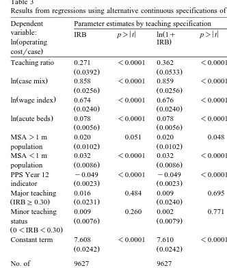
Table 3
Results from regressions using alternative continuous specifications of teaching intensity variables Dependent Parameter estimates by teaching specification
variable: IRB p)< <t ln 1qŽ p)< <t ln 0.001qŽ p)< <t
Ž . .
ln operating IRB IRB
.
costrcase
Teaching ratio 0.271 -0.0001 0.362 -0.0001 0.0196 -0.0001
Ž0.0392. Ž0.0533. Ž0.00442.
Ž .
ln case mix 0.858 -0.0001 0.859 -0.0001 0.867 -0.0001
Ž0.0256. Ž0.0256. Ž0.0257.
Ž .
ln wage index 0.674 -0.0001 0.676 -0.0001 0.681 -0.0001
Ž0.0240. Ž0.0240. Ž0.0241.
Ž .
ln acute beds 0.078 -0.0001 0.078 -0.0001 0.078 -0.0001
Ž0.0056. Ž0.0056. Ž0.0058.
PPS Year 12 y0.049 -0.0001 y0.049 -0.0001 y0.049 -0.0001
Ž . Ž . Ž .
indicator 0.0023 0.0023 0.0023
Major teaching 0.016 0.484 0.009 0.695 0.039 0.181
ŽIRBG0.30. Ž0.0231. Ž0.0240. Ž0.0290.
Minor teaching 0.009 0.260 0.002 0.771 y0.064 0.018
Ž . Ž . Ž .
status 0.0076 0.0079 0.0187
Ž0-IRB-0.30.
Constant term 7.608 -0.0001 7.610 -0.0001 7.743 -0.0001
Ž0.0242. Ž0.0242. Ž0.0421.
Smearing estimates: mean of exponentiated residuals :
In full sample 1.045 1.045 1.046
In teaching only 1.043 1.043 1.044
In non-teaching 1.053 1.054 1.053
ŽWeighted Least Squares with Huber–White adjustment; robust standard errors appear in parentheses ..
these continuous specifications track closely with the results from the dummy variable model, until the highest two groups. The number of observations in these
Ž .
estimates for either of these two groups, and the same pattern was present in each of the two years when we examined them separately.
From the third frame in Fig. 2, it is evident that the logarithm function based on
Ž0.001qIRB produces a substantial distortion in the teaching effect when it is.
restricted to a single slope coefficient for both minor and major teaching hospitals.
Ž
Strong marginal effects are estimated for hospitals with very low ratios less than
.
0.02 while increments above 0.10 produce little or no change in the cost differentials. Although the indicator variables for minor and major teaching status mitigate the distortion somewhat, the function does not approximate the results from the semi-parametric model.
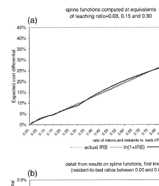
This distortion is an artifact of the log transformation that gives additional influence to the smaller values in the distribution, and it can be corrected by relaxing the assumption of a single slope in the log form. Results from piecewise
Ž .
regression using spline functions are plotted in Fig. 3 a and show that once multiple slope coefficients are allowed, substantive differences in the estimated teaching effects across the three specifications appear only at very low and very
Ž .
high ratios. Fig. 3 b provides greater detail for IRB values below the first spline knot. F-tests for the equality of the spline coefficients indicate that for variables
Ž .
constructed from ln 0.001qIRB , slopes are significantly different beginning with the knot at IRB)0.15 and again at IRB)0.30. There are no significant differ-ences between slopes, however, when the spline functions are constructed from
Ž .
IRB without transformation, or from ln 1qIRB .
4.2. Isolating retransformation effects
Smearing factors that are computed from the estimation sample as a whole are between 1.045 and 1.046 for all of our specifications, from which we can conclude that failure to account for error retransformation in any given prediction would result in an understatement of predicted cost by 4% to 5%. Smearing factors were also computed separately from the residuals within each teaching hospital sub-group for which the model identified different slopes andror intercepts. Factors computed within hospital sub-groups follow similar patterns across all
specifica-Ž
tions. The ratios of smearing factors teaching hospital subgroups divided by
.
non-teaching hospitals range only from 0.99 to 1.02. In comparing our ratios to those computed by Rogowski and Newhouse for hospitals grouped by low, medium and high tertiles of IRB, we find that ours are smaller. Further, we find that they are not similarly above or below 1.00; that is, the implied retransforma-tion correcretransforma-tions to the payment formula are not necessarily in the same direcretransforma-tion as those computed by Rogowski and Newhouse.
The estimated cost differentials that were plotted in Fig. 3 were simplified by assuming that the smearing estimates for the teaching and non-teaching hospitals
Ž
Fig. 3. Expected teaching cost differentials computed from spline functions, across alternative
Ž . Ž .
continuous specifications of the teaching ratio. a Showing all ranges of IRB. b Expanded to show range below lowest spline knot.
.
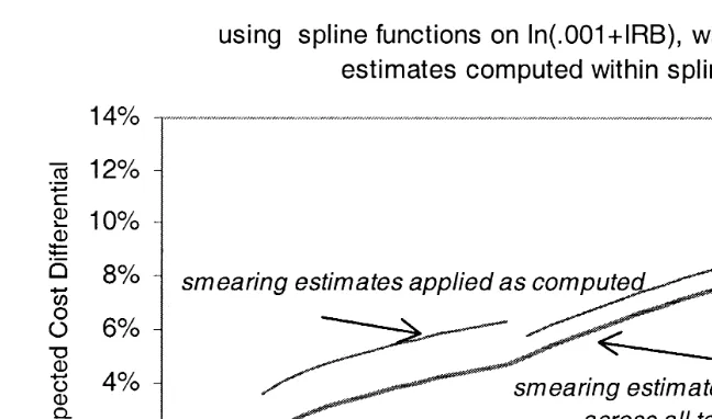
cancelled each other out and have had no effect the calculation . When we include the actual smearing estimates in the calculations, discontinuities are introduced to the regression results. Fig. 4 illustrates this using the piecewise linear regression
Ž .
Ž
Fig. 4. The effects of smearing estimates on expected teaching cost differentials computed for
.
low-to-mid ranges of the teaching ratios only .
In the categorical model the smearing ratio from the first dummy variable group is 1.008, but including this factor in the computation increases the teaching adjustment from 1.6% to 2.4%. In the same model, the smearing ratio from the tenth group is 0.995, and including this factor lowers the adjustment from 25.8% to 25.2%. Although the proportional effects are small in the larger teaching programs, the dollar impact would still be quite large, as these hospitals have the highest IME adjustment rates and the highest volume of Medicare cases.
Given the magnitude of the impact of these corrections on both distribution and total level of IME payments, a formal test of the assumption of heteroscedasticity is in order. We repeated one of Rogowski and Newhouse’s tests for non-constant variance by regressing the exponentiated residuals on a constant plus sets of dummy variables reflecting hospital sub-groups as they were defined in each of our specifications. In each case, the coefficients on the dummy variables tested individually and jointly non-significant. The F-statistic for the joint null
hypothe-Ž .
sis on the dummy variable model was FŽ11,9615.s0.26 ps0.99 ; on splines from
Ž . Ž .
IRB, FŽ4,9621.s0.69 ps0.63 ; on splines from ln 1qIRB , FŽ4,9621.s0.68
Žps0.64 ; on splines from ln 0.001. Ž qIRB , F. Ž4,9621.s0.53 Žps0.75 . In con-.
Ž .
4.3. SensitiÕity to omittedÕariables and outlier cases
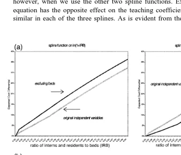
We are interested in whether any of our specifications appears to be less sensitive than the others to added variables or to extreme values or influential observations. All of the specifications of the hospital cost function suffer from omitted variable bias. For example, in the model using splines derived from
Ž .
ln 0.001qIRB , at an IRB of 0.25, adding controls for Medicaid utilization, census region and ownership decreases the estimated teaching cost differentials by
Ž .
3.1 percentage points from 7.6% to 4.5% . Similar increments are computed, however, when we use the other two spline functions. Excluding beds from the equation has the opposite effect on the teaching coefficients, but again, effect is similar in each of the three splines. As is evident from the four frames in Fig. 5,
Fig. 5. Comparing sensitivity to omitted variable bias by choice of log-transformation on the teaching
Ž . Ž .
the spline versions of both log–log models are sensitive to the exclusion or inclusion of key hospital characteristics. There does appear to be some difference in sensitivity to added variables between the single slope and the multiple slope
Ž .
formulations on the ln 1qIRB , but it is not consistent; at lower IRB levels the single-slope estimates are less sensitive, while at higher levels they are more sensitive.
Our results contrast sharply to what Rogowski and Newhouse found in similar variations. They estimated, for example, that excluding beds from the original
Ž .
single slope model using ln 1qIRB increased the cost differentials by 3.5 percentage points. Yet when they excluded beds from a model using their final re-formulation of the teaching variable, estimated teaching differentials increased by only 0.8 percentage points.
All of our models are similar in predictive ability, with R2 between 0.76 and
0.77, with or without the added variables. This is not surprising, as over 70% of variation in logged operating cost per case can be explained by case mix and wage index values alone. Although this is an improvement over the explained variance
Ž .
in the estimations on 1984 data from 0.65 to 0.68 the most likely explanation for this improvement is reduced measurement error in the teaching, case-mix and wage index measures over this period. Refining the model with additional explanatory variables alters the parameter estimates on the original covariates, but it has little effect on predicted costs. We do not, however, address the conceptual or policy motivations for HCFA’s decision to restrict the model’s covariates; see
Ž .
Sheingold 1990 .
Examination of the residuals revealed few differences among the three continu-ous teaching variable models once multiple slope coefficients were introduced. In all cases outlier observations were predominantly non-teaching hospitals-either very small institutions or high-cost specialty facilities, with extreme values in the dependent variable. Because cost per case has been logged, their impact on the model is already minimized and predicted results are not sensitive to their inclusion in the estimation sample. High leverage observations tended to be more evenly distributed across the sample by teaching status. Considering the immediate policy applications of this model, we are more interested in identifying observa-tions with undue influence on the teaching coefficient than on predicted values. We examined sensitivity to extreme values in the explanatory variable of interest
Ž
by excluding the few observations at the far right of the IRB distribution above
.
1.0 . This change had only a slight effect on the teaching coefficient in the exponential model and negligible effects on the logged specifications. We also
Ž
constructed a wage and case-mix adjusted cost per case variable thus
standardiz-.
5. Discussion
The differences that we have identified between our findings and those of Rogowski and Newhouse may be due to secular changes in the hospital industry over the period from 1984 to 1995, some of which is evident from the parameter estimates generated on the model’s control variables. These are different in magnitude, significance, and even direction from effects measured on similar variables from other studies using earlier data, including those by Rogowski and Newhouse. In both the original and expanded models, for example, the differen-tials between urban and rural areas have declined sharply and the magnitude of the
Ž
teaching coefficient has declined. In the expanded model regression results
.
available from the authors on request , the coefficients on public and private ownership reversed sign.
While our findings on all continuous teaching variable specifications other than those with the smaller constant indicate that the log-linear effect in 1994–1995 is constant throughout the sample, and that there are no significant fixed differentials for major or minor teaching institutions, this was not true in earlier critiques of the
Ž .
cost function Welch, 1987; Thorpe, 1988 . More recently, a panel study con-ducted by the authors with data from 1989 through 1995 identified significant positive interaction effects between teaching intensity and both teaching status and
Ž .
DSH eligibility, when measured across the seven-year period Dalton et al., 2000 . The strength of the interactions declined over time, however, and they are no longer significant by the last years of data.
In the Rogowski and Newhouse study it is not possible to separate the effect of allowing multiple slope coefficients from the effects of altering the log transforma-tion, since multiple slopes were not tested under the other formulations of the teaching variable. Thus, the improved stability that they noted in their model may be attributable to the generalization of the log-linear form through the spline functions-during a period when the slope coefficients were truly different-rather than to the use of the smaller constant.
intensity. In that case their formulation of the teaching variable using splines
Ž .
derived from ln 0.0001qIRB would have corrected an underlying error in the functional form of the HCFA model, but for reasons relating to the spline formulation rather than the use of a smaller constant.
From the results on the model using dummy variables, we do not identify a threshold below which no significant teaching effect exists. Cost differentials for hospitals with ratios below 0.07 are small but marginally significant. Models using a continuous teaching measure with multiple slopes consistently produce non-sig-nificant coefficients at very low IRB values. There may, however, be insufficient variation in the lower ranges of the ratio to identify the effect in a continuous measure, despite the large number of observations in these groups. From the plotted results of the dummy variable model we can also see that an assumption of decreasing marginal effect in the higher ranges of the teaching ratio appears more likely to fit the data than one of increasing marginal effect, even though the small number of observations with ratio values above 0.70 prevents us from rejecting the exponential model on the basis of statistical tests. HCFA currently uses an exponential model to compute IME adjustments to the capital portion of the PPS payment, based on the ratio of residents to average daily census. If an exponential model were used to compute adjustments for both the operating and capital components of the per-case payments, it would produce substantially higher payments for a small group of hospitals with very large teaching programs. We do not, however, find any empirical evidence that the exponential model represents an improvement over the original logarithmic one. Results from the semi-parametric model might even suggest an adjustment formula that is derived from either the
Ž .
IRB or ln 1qIRB , but is capped at some maximum value around 0.70 or 0.80. Finally, our findings indicate that including separate smearing estimates in the computation of expected teaching cost differentials is unnecessary. Although variance correction factors are appropriate to retransformation of logged model results, unless there are systematic differences in the distribution of the error term across groups of teaching hospitals, the factors will cancel each other out in the IME payment formula. We find no evidence of such systematic differences in our data. Rogowski and Newhouse correctly identified the retransformation error that was present in HCFA’s interpretation of the teaching coefficient, in light of the significant groupwise heteroscedasticity that they identified in 1984 data. There-fore, because this issue has such a strong potential influence on estimated teaching cost differentials, any future re-estimations of indirect medical education costs should continue to test for this type of non-constant variance.
Acknowledgements
References
Anderson, G.F., Lave, J.R., 1986. Financing graduate medical education using multiple regression to set payment rates. Inquiry 23, 191–199.
Dalton, K., Norton, E.C., Kilpatrick, K.E., 2000. A longitudinal study of the effects of graduate medical education on hospital operating costs. Health Services Research, forthcoming.
Duan, N., 1983. Smearing estimate: a nonparametric retransformation method. Journal of the American
Ž .
Statistical Association 78 383 , 605–610.
Kennedy, P., 1981. Estimation with correctly interpreted dummy variables in semilogarithmic equa-tions. American Economic Review 71, 801.
Lave, J.R., 1985. The Medicare Adjustment for the Indirect Costs of Medical Education: Historical Development and Current Status. Association of American Medical Colleges, Washington, DC. Manning, W.G., 1998. The logged dependent variable, heteroscedasticity, and the retransformation
Ž .
problem. Journal of Health Economics 17 3 , 283–296.
MedPAC, 1999. Report to the Congress: Rethinking Medicare’s Payment Policies for Graduate Medical Education and Teaching Hospitals. Washington, D.C.: Medicare Payment Advisory Commission.
Pettengill, J., Vertrees, J., 1982. Reliability and validity in hospital case-mix measurement. Health Care
Ž .
Financing Review 4 2 , 101–127.
Phillips, S.M., 1992. Measuring teaching intensity with the resident-to-average daily census ratio.
Ž .
Health Care Financing Review 14 2 , 59–68.
Rogowski, J.A., Newhouse, J.P., 1992. Estimating the indirect costs of teaching. Journal of Health Economics 11, 153–171.
Sheingold, S.H., 1990. Alternatives for using multivariate regression to adjust prospective payment
Ž .
rates. Health Care Financing Review 11 3 , 31–41.
Thorpe, K.E., 1988. The use of regression analysis to determine hospital payment: the case of medicare’s indirect teaching adjustment. Inquiry 25, 219–231.