Geomorphological Analysis and Hydrological Potential Zone
of Baira River Watershed, Churah in Chamba District of
Himachal Pradesh, India
Kuldeep Pareta1* and Upasana Pareta21Head (Engineering & Planning Division), ACPL Global Pvt. Ltd., Kanpur (U.P.), India
2Department of Mathematics, PG Collage, District Sagar (M.P.) India
*Correspondence: E-mail: [email protected]
A B S T R A C T S A R T I C L E I N F O
In the present study, an attempt has been made to study the quantitative geomorphological analysis and hydrological characterization of 95 micro-watersheds (MWS) of Baira river watershed in Himachal Pradesh, India with an area of 425.25 Km2. First time in the world, total 173 morphometric parameters have been generated in a single watershed using satellite remote sensing data (i.e. IRS-P6 ResourceSAT-1 LISS-III, LandSAT-7 ETM+, and LandSAT-8 PAN & OLI merge data), digital elevation models (i.e. IRS-P5 CartoSAT-1 DEM, ASTER DEM data), and soI topographical maps of 1: 50,000 scale. The ninety-five micro-watersheds (MWS) of Baira river watershed have been prioritized through the morphometric analysis of different morphometric parameters (i.e. drainage network, basin geometry, drainage texture analysis, and relief characterizes ). The study has concurrently established the importance of geomorphometry as well as the utility of remote sensing and GIS technology for hydrological characterization of the watershed and there for better resource and environmental managements.
© 2017 Tim Pengembang Jurnal UPI
Article History:
Received 03 January 2017 Revised 12 January 2017 Accepted 17 February 2017 Available online 01 April 2017 ____________________ Keyword:
Geomorphometric analysis, hydrological characterization, remote sensing and GIS analysis, micro-watershed assessment.
Indonesian Journal of Science & Technology
1. INTRODUCTION
Geomorphometry is the science ''which treats the geometry of the landscape", and quantitative procedure of the land surface.(Chorley et al., 1957) Morphometry is the quantitative analysis of the conformation of the earth's surface, shape and dimension of its landforms. The field of geomorphology fundamentally characterizes the topographical appearance of land by way of area, slope, shape, length, etc. A major highlighting in geomorphology over the past several decades has been on the development of quantitative physiographic methods to describe the evolution and behavior of surface drainage networks (Horton, 1945; Abrahams, 1984).
Some quantitative approaches have been documented to identify the basin drainage characteristics, and for sympathetic of various hydrological processes. The morphometric characteristics at the watershed scale may contain important information regarding its formation development and spatio-temporal variations because all hydrologic and geomorphic processes occur within the watershed. The quantitative measurement of landforms has become the current trust of geomorphology. Earlier, it has been well attempted by various hydrologists, geologists and geomorphologists. (Horton, 1932; Horton, 1945; Potter, 1957; Schumm, 1956; Mueller, 1968; Sutherland & Bryan, 1991; Rahmat & Mutolib, 2016) Morphometry is potentially a most important approach to geomorphology, since it affords quantitative information on large scale fluvial landforms, which make up the vast majority of earth configuration.
Micro-watershed is the fundamental unit in hydrology; consequently, geomorphometric analysis at micro-watershed scale is helpful and better rather carries it out on completes it on particular
channel or inconsistent segment areas. Hydrologic and geomorphic strategies happen contained by the watershed, and morphometric characterization at the watershed scale reveals data considering formation and improvement of land exterior methods (Dar et al., 2013) and thusly is responsible of a comprehensive comprehension into the hydrologic behaviour of a watershed. Additionally, some of the morphometric parameters, for example, circularity proportion and bifurcation ratio are input parameters in the hydrograph examination (Jain et al., 2000;
Angillieri, 2008) and assessment of surface water capability of an area (Suresh et al., 2004). In this point of view, this study covers a better thoughtful of hydrologic conduct of the study area and the geomorphometric analysis of micro-watersheds (MWS) for hydrological scenario evaluation and characterization Baira river watershed, Churah in Chamba district of Himachal Pradesh, India.
2. MATERIALS AND METHODS
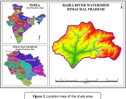
DOI: http://dx.doi.org/10.17509/ijost.v2i1 p- ISSN 2528-1410 e- ISSN 2527-8045 3. RESULTS AND DISCUSSION tehsil of Chamba district at a height of 5268 m, flows towards south, south-east and finally joins the river Makkan at Buin village of Chaurah tehsil of Chamba district in Himachal Pradesh. Baira river is 19.07 Kms long, however there is only one main tributaries of the right bank of Baira river i.e. Malin Nadi, there are some major tributaries pouring into the left bank river, notable amongst there are Cheni Nala, Trishan Nala, Tabriyali Nala, Bhusandu Nala and Chhawed Nala. The study area falls in Survey of India
(1:50,000) toposheets No. 52C/04 (I 3Q/04), 52 /08 (I43Q/08), 52D/01 (I43W/01) and 52D/05 (I43W/05). According to new watershed codification system (Pareta & Pareta, 2014), total 95 micro-watershed (MWS) has covered the whole study area.
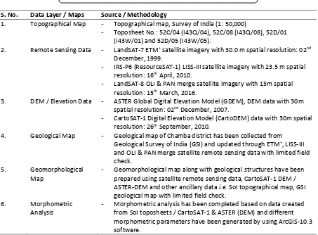
3.2. DATA USED, SOURCES AND METHODOLOGY
Different type of data has been used for this study. Data from satellite remote
1. Topographical Map - Topographical map, Survey of India (1: 50,000)
- Toposheet No.: 52C/04 (I43Q/04), 52C/08 (I43Q/08), 52D/01 (I43W/01) and 52D/05 (I43W/05).
2. Remote Sensing Data - LandSAT-7 ETM+ satellite imagery with 30.0 m spatial resolution: 02nd December, 1999.
- IRS-P6 (ResourceSAT-1) LISS-III satellite imagery with 23.5 m spatial resolution: 16th April, 2010.
- LandSAT-8 OLI & PAN merge satellite imagery with 15m spatial resolution: 15th March, 2016.
3. DEM / Elevation Data - ASTER Global Digital Elevation Model (GDEM), DEM data with 30m spatial resolution: 02nd December, 2007.
- CartoSAT-1 Digital Elevation Model (CartoDEM) data with 30m spatial resolution: 26th September, 2010.
4. Geological Map - Geological map of Chamba district has been collected from Geological Survey of India (GSI) and updated through ETM+, LISS-III and OLI & PAN merge satellite remote sensing data with limited field check.
5. Geomorphological Map
- Geomorphological map along with geological structures have been prepared using satellite remote sensing data, CartoSAT-1 DEM / ASTER-DEM and other ancillary data i.e. SoI topographical map, GSI geological map with limited field check.
6. Morphometric Analysis
- Morphometric analysis has been completed based on data created from SoI toposheets / CartoSAT-1 & ASTER (DEM) and different morphometric parameters have been generated by using ArcGIS-10.3 software.
3.3. WATERSHED CODIFICATION SYSTEM
For this study, authors have been used the watershed codification system proposed by the (Pareta & Pareta, 2014). They have
lassified e ti e i e s i I dia as I dia
sub-continent largest transboundary
ate sheds, ate di isio s, ate
sub-di isio s, asi s, su -basins,
ate sheds a d the i o
classification as sub-watersheds, micro-watershed (MSW), mini-micro-watershed (Mini-WS).
According to them, the study area watershed is situated in the international
ha el. The ate di isio ’s ode is A all
drainage flowing into Arabian sea (A),
A“ I dus i e ; ate su -divisions code
is A all d ai age flo i g i to A a ia sea f o o th I dia; asi ode is Id fo I dus
river; sub- asi ode is RVI fo Ra i i e . They have classified the entire Ravi
sub-asi i to ajo ate sheds i.e. AS11A1Id(RVI)1 to AS11A1Id(RVI)8. They study area is located in the major watershed of AS11A1Id(RVI)7. This watershed future
has lassified i to su -watersheds and symbolized as AS11A1Id(RVI)7a to AS11A1Id(RVI)7l. Authors have selected 3 sub-watersheds namely AS11A1Id(RVI)7d, AS11A1Id(RVI)7e and AS11A1Id(RVI)7f for this study. Under the above stated
sub-ate sheds total i o-watershed has been identified and shown in Fig. 2. The completed code for a micro-watershed with eight digits is represented as
A“ A Id RVI f , as a e a ple of a
micro-watershed of Ravi sub-basin, where
A“ ep ese ts I dia “u -Continent
La gest T a s ou da , A fo Wate Di isio , fo Wate “u -Di isio , Id fo
Basi , RVI fo “u -Basi , fo Watershed, f fo “u -Wate shed, a d for Micro-Watershed.
DOI: http://dx.doi.org/10.17509/ijost.v2i1 p- ISSN 2528-1410 e- ISSN 2527-8045 3.4. GEOLOGY
A systematic geomorphic study has been attempted for the terrain classification and their significance with the aid of satellite imagery, digital terrain model and surface characters in the study area. Presently, the knowledge of the geomorphology of the region is very sketchy and hence an appraisal of terrain types, drainage basin, river valleys and the morphometric study to understand the history of geomorphic evolution in this part of the Himalayan belt has been brought out to assist in the study basin management. The gamut of geomorphic description of study area in the region initially dictates the need for understanding the geologic events reflecting the relief and hence the paper highlights first the rock description along with their influence on basin management.
Various folks are studies the geological aspects of the study area (Tomlinson, 1925;
De Terra, 1939; Krishnan & Aiyengar, 1940;
Woodroffe, 1981; Boison & Patton, 1985). They have recorded the primary rock formations namely (i) Chamba Formation: Slate, Phyllite Carbonaceous Slate and Quartzite; (ii) Katarigali Formation: Dark Grey Slate, Micaceous Sandstone and Quartzite; and (iii) Manjir Formation: Slate, Shale, Sandstone and Limestone. The mountain blocks in the study area are composed of a series of differing architectural elements represented by sedimentary, metamorphosed sediments and igneous massifs in the following tectonic sequence. The study area lies between the two high mountain ranges, i.e. the Dhauladhar Range in the southwest and the Zanskar Range or the Great Himalayan Range in the northwest. Stratigraphic sequence of the study area is shown in Table 2.
Age Group Formation Lithology
Neoproterozoic - Katarigali Dark Grey Slate, Micaceous Sandstone and Quartzite Manjir Slate, Shale, Sandstone and Limestone
Undifferentiated Proterozoic Vaikrita Chamba Slate, Phyllite Carbonaceous Slate and Quartzite Source: Geological Survey of India (GSI)
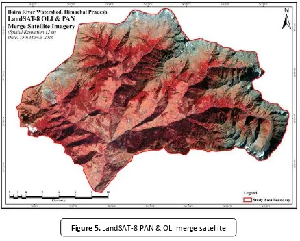
3.5. METHOD FOR GEOLOGICAL MAPPING
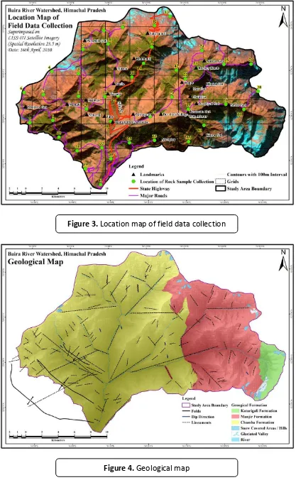
The methods adopted for this research work is divided into two aspects namely field and lab operations. The field operation is essentially geologic mapping of the study area to determine the underlying lithologic units. The geologic mapping was carried out at a scale of 1:50,000 using grid-controlled sampling method at a sampling density of one sample per 9 km2 for the collection of stream sediments and rock samples. The location map of field data collection is shown in Figure 3. Total fourty-three (43) rock and stream sediment samples were obtained. The rock samples were collected from different localities in the studied area, after which they were labelled accordingly to avoid mix up. The geographical location of each outcrop was determined with the aid of a Global Positioning Systems (GPS) and the lithologic and field description and features characteristic of each sample were correctly recorded in the field notebook. Six distinct lithological units were recognized in the studied area which were compiled to
produce a geological map, which are the slate, micaceous sandstone, quartzite, shale, phyllite carbonaceous slate and limestone. The major structure in the area is an anticline, syncline, fault, fractures, joints and lineaments, which are visible on the lithology in the studied area.
For lab operations, a published geological map from Geological Survey of India (GSI) has been used for preparation of geological map of the study area. This geological map has been update through the satellite remote sensing data i.e. LandSAT-7 ETM+, (30m) IRS-P6 (ResourceSAT-1) LISS-III (23.5), LandSAT-8 OLI & PAN merge (15m), CartoSAT-1 (DEM) data (30m), ASTER (DEM) data (30m) by using ESRI based ArcGIS-10.3 software along with comprehensive field work as described above. Other ancillary data like Survey of India (SoI) topographical map at 1:50,000 scales has also used. The above stated data has been used for identification of various geological parameters and lithology of the study area. The detailed geological map of the study area is shown in Figure. 4.
Tabel 2. Stratigraphic sequence of baira river watershed, himachal pradesh
DOI: http://dx.doi.org/10.17509/ijost.v2i1 p- ISSN 2528-1410 e- ISSN 2527-8045 Figure 3. Location map of field data collection
3.6. APPLIED GEOMORPHOLOGY
The term of applied geomorphology implies the utilization of our geomorphological information in fervor of the general public or the humankind in general. This science demonstration like a bridge to some of the gaps that have segregated the several disciplines of the geomorphology. It covers those aspects of the geomorphology that are specifically related with environment issues and decision making processes which are of value of agricultural researchers, engineers, geologists and hydrologists and in addition geomorphologists.
The key application of geomorphology in the study area has been observed. for example, soil erosion, various types of slope failure, river floods, volcanoes, earth-quakes and faulting as natural hazards. Now and then we found the result of the utilization of main procedures impulsively somehow, specifically, if there is an occurrence of soil
erosion and man-made problem.
Earthquakes (natural problems) in such conditions can be the role of expert geomorphologist that comes in picture since they would be able to measure of comprehension of the combinations of occasions that created the hazards.
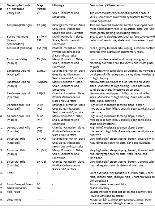
Satellite remote sensing data, aerial photographs, digital elevation model and digital terrain model is an important tool for preparation of geomorphological map. The geomorphological map is can be prepared from small scale 1:1 million to a larger scale of 1:1,000 but it is depending on the scope, scale, purpose and nature of problems the geomorphological map. The detailed geomorphological map of the study area has been prepared through visual image interpretation of satellite data (i.e. IRS-P6 ResourceSAT-1 LISS-III, LandSAT-7 ETM+ and LandSAT-8 PAN & OLI merge data) (See component were identified and mapped (Figure 6). The important geomorphic units, their lithology and description/ characteristics are shown in Table 3.
3.7. MORPHOMETRIC ANALYSIS
Horton and Strahler were the first geomorphologists, who measured the various morphometric parameters of river basin. (Horton, 1945; Strahler, 1952) Morphometric analysis is the mathematical measurement of configuration of the earth surface, shape, and dimension of its landforms in a given drainage basin. Landforms and morphometric analyses are significant in the study of geomorphology with the quantitative measurements of physical characteristics of landforms to understand the structure, processes and evolution of landscape. It is also help to comprehension the hydrological behavior of drainage basin and controlled the predominantly climate, geology, geomorphology, structural backgrounds of the river basin.
The morphometric characteristics at the river basin scale may contain essential information in regards to its formation and development since all hydrologic and geomorphic processes occur within the river basin. The relationship between various morphometric parameters and the above-mentioned factors are well recognized by various geomorphologists (Rich, 1916;
Wenthworth, 1930; Horton, 1932; Strahler, 1952; Taylor & Schwarz, 1952; Potter, 1957;
Schumm, 1956; Chorley, 1957; Hack, 1957;
DOI: http://dx.doi.org/10.17509/ijost.v2i1 p- ISSN 2528-1410 e- ISSN 2527-8045
Surkan, 1967; Faniran, 1968; Mueller, 1968;
Black, 1972; Moore & Thornes, 1976; Patton & Baker, 1976; Pareta, 2004). They have documented that relations are very significant between hydrological characteristics, geological and geomorphic characteristics of river basin system. Several key hydrologic phenomena can be linked with the physiographic characteristics of river basin such as size, shape, geometry, drainage density, relief, slope of drainage area, size and length of the contributories etc. (Rastogi & Sharma, 1976). The quantitative analysis of morphometric parameters is found to be of huge utility in river basin evaluation, watershed prioritization for soil and water conservation and natural resources management. The morphometric analysis of the Baira river watershed has been carried out based on satellite remote sensing data (i.e. IRS-P6
ResourceSAT-1 LISS-III, LandSAT-7 ETM+ and LandSAT-8 PAN & OLI merge data), digital elevation models (i.e. IRS-P5 CartoSAT-1 DEM, ASTER DEM data), and soI topographical maps of 1: 50,000 scale. The drainage network with stream order has been generated by using above stated DEM data and rectified its using SoI topographical maps through ArcGIS-10.3 software. Stream ordering has been generated using (Strahler, 1952) system, and ArcHydro tool in ArcGIS-10.3 software. First time in the world, authors have investigated O e-Hundred
and Seventy-Three Morphometric
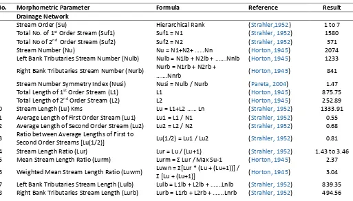
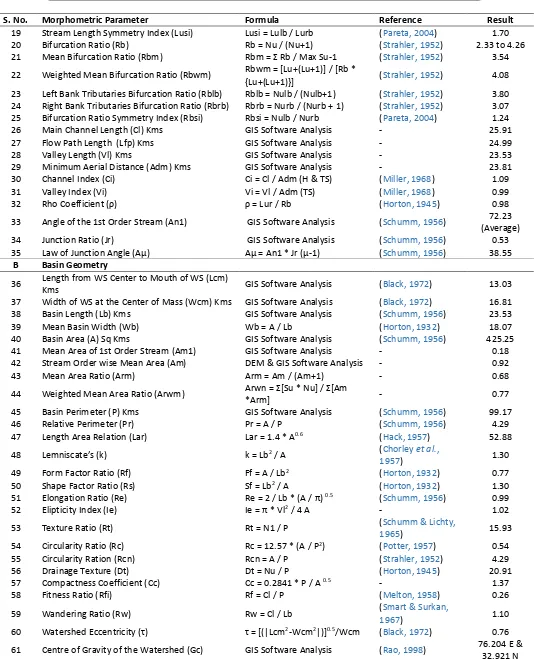
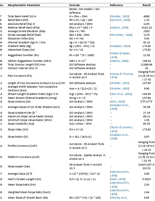
Pa a ete s of a single watershed. Out of 173 parameters, 54 morphometric parameters have been directly analysed and generated in ArcGIS-10.3 software. Morphometric parameters of Baira river watershed with formula, references and result are shown in Table 4.
S.
No. Geo orphi U its or La dfor s Map Sy ol Lithology Des riptio / Chara teristi . Valley Fills VF “hale, “a dsto e a d
Li esto e The unconsolidated sediment deposited to fill a valley, sometimes controlled by fracture forming linear depression. sides. Mode ate to high slopi g. Deep sites ith sa d, slate, shale, li esto e o upla ds.
. “a dsto e Upla d
Cha a ““T CB Cha a Fo atio : “late, Ph llite Ca o a eous
“late a d Qua tzite
Na o sites o slopes of hills, s a ps a d alle sides. Mode ate to high slopi g. Deep sites ith slate, sa d, ua tzite.
Ph llite “late a d Qua tzite.
. Li ea e ts --- - F a tu es, joi ts, shea zo e, o ta t zo es, othe
DOI: http://dx.doi.org/10.17509/ijost.v2i1 p- ISSN 2528-1410 e- ISSN 2527-8045
S. No. Morphometric Parameter Formula Reference Result
A Drainage Network
1 Stream Order (Su) Hierarchical Rank (Strahler,1952) 1 to 7
2 Total No. of 1st Order Stream (Suf1) Suf1 = N1 (Strahler, 1952) 1580 3 Total No of 2nd Order Stream (Suf2) Suf2 = N2 (Strahler, 1952) 371
4 Stream Number (Nu) Nu = N +N + ……N (Horton, 1945) 2074
5 Left Bank Tributaries Stream Number (Nulb) Nul = N l + N l + …….N l (Horton, 1945) 1233
6 Right Bank Tributaries Stream Number (Nurb) Nurb = N1rb + N2rb +
…….N (Horton, 1945) 841
7 Stream Number Symmetry Index (Nusi) Nusi = Nulb / Nurb (Pareta, 2004) 1.47 8 Total Length of 1st Order Stream (L1) L1 (Horton, 1945) 875.75 9 Total Length of 2nd Order Stream (L2) L2 (Horton, 1945) 252.89
10 Stream Length (Lu) Kms Lu = L +L …… L (Strahler, 1952) 1333.91
11 Average Length of First Order Stream (Lu1) Lu1 = L1 / N1 (Strahler, 1952) 0.55 12 Average Length of Second Order Stream (Lu2) Lu2 = L2 / N2 (Strahler, 1952) 0.68
13 Ratio between Average Lengths of First to
Second Order Streams [Lu(1/2)] Lu(1/2) = Lu1 / Lu2 (Strahler, 1952) 0.81 14 Stream Length Ratio (Lur) Lur = Lu / (Lu+1) (Strahler, 1952) 1.43 to 3.46 15 Mean Stream Length Ratio (Lurm) Lu = Ʃ Lu / Ma “u-1 (Horton, 1945) 2.37
16 Weighted Mean Stream Length Ratio (Luwm) Lu = Ʃ[Lu * Lu + Lu+ ] / Ʃ [Lu + Lu+ ] (Horton, 1945) 3.04
17 Left Bank Tributaries Stream Length (Lulb) Lul = L l + L l + …….L l (Strahler, 1952) 839.35 18 Right Bank Tributaries Stream Length (Lurb) Lu = L + L + …….L (Strahler, 1952) 494.56
Tabel 4. (continued) Comparison of drainage basin characteristics of Baira river
watershed Watershed conditions Figure 6. Geomorphological map
S. No. Morphometric Parameter Formula Reference Result
19 Stream Length Symmetry Index (Lusi) Lusi = Lulb / Lurb (Pareta, 2004) 1.70 20 Bifurcation Ratio (Rb) Rb = Nu / (Nu+1) (Strahler, 1952) 2.33 to 4.26 21 Mean Bifurcation Ratio (Rbm) R = Ʃ R / Ma “u-1 (Strahler, 1952) 3.54
22 Weighted Mean Bifurcation Ratio (Rbwm) Rbwm = [Lu+(Lu+1)] / [Rb *
{Lu+(Lu+1)}] (Strahler, 1952) 4.08 23 Left Bank Tributaries Bifurcation Ratio (Rblb) Rblb = Nulb / (Nulb+1) (Strahler, 1952) 3.80 24 Right Bank Tributaries Bifurcation Ratio (Rbrb) Rbrb = Nurb / (Nurb + 1) (Strahler, 1952) 3.07 25 Bifurcation Ratio Symmetry Index (Rbsi) Rbsi = Nulb / Nurb (Pareta, 2004) 1.24
26 Main Channel Length (Cl) Kms GIS Software Analysis - 25.91
27 Flow Path Length (Lfp) Kms GIS Software Analysis - 24.99
28 Valley Length (Vl) Kms GIS Software Analysis - 23.53
29 Minimum Aerial Distance (Adm) Kms GIS Software Analysis - 23.81
30 Channel Index (Ci) Ci = Cl / Adm (H & TS) (Miller, 1968) 1.09
31 Valley Index (Vi) Vi = Vl / Adm (TS) (Miller, 1968) 0.99
32 Rho Coeffi ie t = Lu / R (Horton, 1945) 0.98
33 Angle of the 1st Order Stream (An1) GIS Software Analysis (Schumm, 1956) 72.23 (Average) 34 Junction Ratio (Jr) GIS Software Analysis (Schumm, 1956) 0.53
35 La of Ju tio A gle Aμ Aμ = A * J μ-1) (Schumm, 1956) 38.55
B Basin Geometry
36 Length from WS Center to Mouth of WS (Lcm)
Kms GIS Software Analysis (Black, 1972) 13.03
37 Width of WS at the Center of Mass (Wcm) Kms GIS Software Analysis (Black, 1972) 16.81 38 Basin Length (Lb) Kms GIS Software Analysis (Schumm, 1956) 23.53
39 Mean Basin Width (Wb) Wb = A / Lb (Horton, 1932) 18.07
40 Basin Area (A) Sq Kms GIS Software Analysis (Schumm, 1956) 425.25 41 Mean Area of 1st Order Stream (Am1) GIS Software Analysis - 0.18 42 Stream Order wise Mean Area (Am) DEM & GIS Software Analysis - 0.92
43 Mean Area Ratio (Arm) Arm = Am / (Am+1) - 0.68
44 Weighted Mean Area Ratio (Arwm) A = Ʃ[“u * Nu] / Ʃ[A
*Arm] - 0.77
45 Basin Perimeter (P) Kms GIS Software Analysis (Schumm, 1956) 99.17
46 Relative Perimeter (Pr) Pr = A / P (Schumm, 1956) 4.29
47 Length Area Relation (Lar) Lar = 1.4 * A0.6 (Hack, 1957) 52.88
48 Le is ate’s k k = Lb2 / A (Chorley et al.,
1957) 1.30
49 Form Factor Ratio (Rf) Ff = A / Lb2 (Horton, 1932) 0.77
50 Shape Factor Ratio (Rs) Sf = Lb2 / A (Horton, 1932) 1.30
51 Elongation Ratio (Re) Re = / L * A / 0.5 (Schumm, 1956) 0.99
52 Elipticity Index (Ie) Ie = * Vl2 / 4 A - 1.02
53 Texture Ratio (Rt) Rt = N1 / P (Schumm & Lichty,
1965) 15.93
54 Circularity Ratio (Rc) Rc = 12.57 * (A / P2) (Potter, 1957) 0.54
55 Circularity Ration (Rcn) Rcn = A / P (Strahler, 1952) 4.29
56 Drainage Texture (Dt) Dt = Nu / P (Horton, 1945) 20.91
57 Compactness Coefficient (Cc) Cc = 0.2841 * P / A 0.5 - 1.37
58 Fitness Ratio (Rfi) Rf = Cl / P (Melton, 1958) 0.26
59 Wandering Ratio (Rw) Rw = Cl / Lb (Smart & Surkan,
1967) 1.10
60 Wate shed E e t i it τ τ = [ |L 2-Wcm2|)]0.5/Wcm (Black, 1972) 0.76
61 Centre of Gravity of the Watershed (Gc) GIS Software Analysis (Rao, 1998) 76.204 E & 32.921 N Tabel 4. (continued) Comparison of drainage basin characteristics of Baira river
DOI: http://dx.doi.org/10.17509/ijost.v2i1 p- ISSN 2528-1410 e- ISSN 2527-8045
S. No. Morphometric Parameter Formula Reference Result
62 Hydraulic Sinuosity Index (Hsi) % Hsi = ((Ci - Vi)/(Ci - 1))*100 (Mueller, 1968) 113.33 63 Topographic Sinuosity Index (Tsi) % Tsi = ((Vi - 1)/(Ci - 1))*100 (Mueller, 1968) -13.33 64 Standard Sinuosity Index (Ssi) Ssi = Ci / Vi (Mueller, 1968) 1.10
65 Longest Dimension Parallel to the Principal
Drainage Line (Clp) Kms GIS Software Analysis - 25.92
66 Area of the Basin to the Right of the Trunk
Stream that Facing Downstream (Ar) Sq Kms GIS Software Analysis - 169.62
67
Distance from the Midline of the Drainage Basin to the Midline of the Active Meander Belt (Damb)
GIS Software Analysis (Cox, 1994) 11.34
68 Distance from the Basin Midline to the Basin
Divide (Dbd) GIS Software Analysis (Cox, 1994) 4.41
69 Area of Left Bank Tributaries (Alb) Sq Kms GIS Software Analysis - 255.63 70 Area of Right Bank Tributaries (Arb) Sq Kms GIS Software Analysis - 169.62
71 Drainage Basin Asymmetry (Bas) Bas = 100 (Ar / A) - 39.89
72 Transverse Topographic Symmetry Factor
(TTSF) TTSF = Damb / Dbd (Cox, 1994) 2.57
73 Ratio of First Order Stream Number to
Perimeter (PN1) PN1 = N1 / P - 15.93
74 Basin Area Symmetry Index (Bsi) Bsi = Alb / Arb (Pareta, 2004) 1.51
75 Valley Width (Vwid) Mts Vwid = Valley width 0.5 Km
from basin mouth - 4.83
76 Meander Width Ratio (MWR) GIS Software Analysis - 1.52
77 Stream Meander Length (Lm) GIS Software Analysis - 23.81
78 Meander Length Ratio (Lmr) Lmr = Lm / MWR - 15.66
79 2D Area of Watershed (A2d) Sq Kms 3D Analyst-Surface Volume
Tool in ArcGIS-10.3 - 423.72
80 3D Arrea of Watershed (A3d) Sq Kms A3d = 2D Area / Cosine (Slope
in degrees) - 527.62
81 Watrshed Volume (Vw) Cubic Meter 3D Analyst-Surface Volume
Tool in ArcGIS-10.3 - 811569.78
C Drainage Texture Analysis
82 Stream Frequency (Fs) Fs = Nu / A (Horton, 1932) 4.88
83 Drainage Density (Dd) Km / Kms2 Dd = Lu / A (Horton, 1932) 3.14
84 Constant of Channel Maintenance (Kms 2 / Km)
89 Flow Direction (Fdi) Spatial Analyst-Hydrology
Tool in ArcGIS-10.3 - NW to SE
90 Flow Accumulation (Range in M) Fac Spatial Analyst-Hydrology Tool in ArcGIS-10.3 -
96 Mean Height Value (Hmv) Summary Statistics for WS - 3206.17
Tabel 4. (continued) Comparison of drainage basin characteristics of Baira river
S. No. Morphometric Parameter Formula Reference Result
Raster; not median / GIS Software
109 Total Contour Length (Ctl) Kms GIS Software Analysis - 12869.96
110 Contour Interval (Cin) m GIS Software Analysis - 20
111 Plan Curvature (Plc) Curvature - 3D Analyst Tools in ArcGIS-10.3 112 Length of Two Successive Contours (L1+L2) Km GIS Software Analysis (Strahler, 1952) 107.95
113 Average Width between Two Successive
Contours (Awc) Awc = A / {(L1+L2) / 2} (Strahler, 1952) 9.90
124 Profile Curvature (CuPr) Curvature - 3D Analyst Tools
in ArcGIS-10.3 -
Ranging from (+) 16.19 to
(-) 18.22
125 Platform Curvature (CuPl) Curvature - Spatial Analyst in
ArcGIS-10.3 -
Ranging from (+) 35.22 to
(-) 31.55
126 Slope Aspect (Sas) 3D Analyst Tools in
ArcGIS-10.3 -
Tabel 4. (continued) Comparison of drainage basin characteristics of Baira river
DOI: http://dx.doi.org/10.17509/ijost.v2i1 p- ISSN 2528-1410 e- ISSN 2527-8045
S. No. Morphometric Parameter Formula Reference Result
1957)
132 Length-Slope Factor (LSf) LSf = 1.4 * [(A/22.13)^0.4] *
[ ta β / . ^ . ] (1992Moore & Wilson, ) 7748.62
133
Topographic Wetness Index (TWI) or Compound Topographic Index (CTI) or Topographic Moisture Index (TMI) or Hillslope Wetness Index (HWI)
TWI = l A / ta β (Moore et al., 1991) 15.00
134 Upslope Contributing Area per Unit Contour
Length (Aus) Aus = Ctl / A (Moore et al., 1991) 30.26
135 Relative Stream Power (SPr) “P = Aus * ta β (Lindsay, 2005) 827.13
136 Stream Power Index (SPI)
“PI = A * ta β o
Topographic Position Index (TPI) or Relative Topographic Position (RTP) or Local Elevation Index (LEI) smtDEM = Name of smoothed elevation raster
138 Slope Position Classification (SPC) Topography Tools in
ArGIS-10.3 (Jenness, 2005)
139 Landform Classification (LC) Topography Tools in
ArGIS-10.3 (Jenness, 2005)
140 Topographic Convergence Index (TCI)
Ln (flow accum+1) /
(tan(((slope Deg.) * 3.141593) / 180))
- 18.99
141 Terrain Characterization Index (TCHi) TCHi = TCI * In Aus (Park et al., 2001) 64.75
142 Length along the Edge of the Mountain
Piedmont Junction (Lmej) GIS Software Analysis - 49.585
143 Overall Length of the Mountain Front (Lmf) GIS Software Analysis - 11.765 144 Mountain Front Sinuosity Index (Simf) Simf = Lmej / Lmf - 4.21
145 Terrain Roughness Index (TRI)
TRI = √ A s F“ a ^ -
((FS3x3max)^2)), where: FS3x3max = Focal statistics of DEM with 3m size / type minimum, FS3x3max = Focal statistics of DEMwith 3m size / type maximum
(Riley, 1999) Highly Rugged
146 Relative Height (h/H) h/H (Strahler, 1952) 100 to 0
Tabel 4. (continued) Comparison of drainage basin characteristics of Baira river
S. No. Morphometric Parameter Formula Reference Result
147 Relative Area (a/A) a/A (Strahler, 1952) 0 to 100
148 Hypsometric Index (HI) HI = (Hmv - Zmi) / (Zmx - Zmi) - 0.50
149 Hypsometric Integral (Hi) % Hypsom Curve h/H & a/A (Strahler, 1952) 58.33 150 Erosional Integral (Ei) % Hypsom Curve h/H & a/A (Strahler, 1952) 41.67
151 Stage of Watershed (WSs) According to Hypsometric
Integral (Strahler, 1952) Mature
152 Clinographic Analysis (Clga) Tan Q = Cin / Awc (Strahler, 1952) 2.02
153 Erosion Surfaces (Es) m Superimposed Profiles (Potter, 1957)
2610, 3130, 3450, 3900 &
4705
154 Surface Area of Relief (Rsa) Sq Kms Composite Profile - 331.77
155 Composite Profile Area (Acp) Sq Kms Area between the Composite
Curve and Horizontal Line (Pareta, 2004) 331.77
156 Minimum Elevated Profile Area as Projected Profile (App) Sq Kms
Area between the Minimum Elevated Profile as Projected Profile and Horizontal Line
(Pareta, 2004) 105.84
157 Erosion Affected Area (Aea) Sq Kms Aea = Acp - App (Pareta, 2004) 225.93 158 Total Soil Loss (SE) [Tonnes/Hectare/Year] TSL = R*K*LS*C*P - 145.12
159 Longitudinal Profile Curve Area (A1) Sq Kms Area between the Curve of the Profile and Horizontal Line
(Snow &
Slingerland, 1987) 122.05
160 Profile Triangular Area (A2) Sq Kms
Triangular Area created by
Slingerland, 1987) 0.58
162 Sediment Transport Capacity Index (STCI) STCI = [1.4 * ((A / 22.13)^0.4)]
* [ ta β / . ^ . ] (Moore et al., 1991) 7748.62
168 Elevation of the Valley Floor or Stream Channel
(Esc) Mts GIS Software Analysis - 1314.00
169 Elevations of the Left Valley Divides (Elvd) Mts GIS Software Analysis - 2783.00 170 Elevations of theRight Valley Divides (Ervd) Mts GIS Software Analysis - 4278.00
171 Valley Floor Width to Valley Height Ratio (Vf) Vf = (2 * Vwid) / ((Elvd - Esc) +
(Ervd - Esc)) - 0.0022
172 Hillslope Erosion Potential (HEP)
HEP = (Pma * S) / 1000,
173 Specific Weight of Sediment Qua tz γs Density relative to Water
(1.65 Constant for Quartz) - 1.65
3.8. CORRELATION ANALYSIS OF DRAINAGE MORPHOMETRIC CHARACTERISTICS
Statistics analyses are useful in a variability of fields in hydrological research.
These analyses are valuable for understanding of morphometric parameters and linking the same to particular hydrological forms. Statistical analysis of Tabel 4. (continued) Comparison of drainage basin characteristics of Baira river
DOI: http://dx.doi.org/10.17509/ijost.v2i1 p- ISSN 2528-1410 e- ISSN 2527-8045 inter-relationship of morphometric
parameters are help to understanding the terrain characteristics for hydrological potential at micro-watershed level as well watershed management and planning.
A correlation matrix Table 5 of Baira river watershed and its 95 micro-watershed (MSW) has been generated with the selected 13 morphometric parameters (i.e. Area (A), perimeter (P), stream number (Nu), stream length (Lu), form factor (Ff), shape factor (Sf), elongation ratio (Re), texture ratio (Rt), circularity ratio (Rc), drainage texture (Dt), stream frequency (Fs), drainage density (Dd), length of overland flow (Lg)). The preliminary observation is confirmed by the statistics as shown in Table 5; furthermost of the morphometric parameters of the Baira river watershed are showing a positive correlation with each other that means these parameters are co-dependent on another, except shape factor and length of overland flow. Shape factor and length of overland flow are demonstrating a negative relationship with other morphometric parameters implies these parameters are independent and it is possible to compelling by different components.
3.9. HYDROLOGICAL POTENTIALITY ZONE
Keeping in mind to identify, categorize, arrange and delineate hydrological potentiality zone in the Baira river watershed, a thorough comprehensive analysis was attempted, which takes several MSW level geo-morphometric parameters map composites into thought by method for integrating and evaluating them based on specific criteria employed. Several thematic data layers have been generated and integrated based on the weightage criteria produced for determination of the hydrological potential zones for surface water, and additionally groundwater investigation in the Baira river watershed. The weightages were relegated to the themes and units relying on their significance of hydrological potentiality area. Hydrological potentiality zones of the Baira river watershed has been generated by using ArcGIS 10.3 software in the model builder module, which has allowed for the amalgamation of different data layers. Weightage criteria used for generation of hydrological potentiality zones are shown in the Table 6.
Where: Area (A), Perimeter (P), Stream Number (Nu), Stream Length (Lu), Form Factor (Ff), Shape Factor (Sf), Elongation Ratio (Re), Texture Ratio (Rt), Circularity Ratio (Rc), Drainage Texture (Dt), Stream Frequency (Fs), Drainage Density (Dd), Length of Overland Flow (Lg)
Factor Values Weights (Wi) Remarks
Bifurcation Ratio (Rb) Less than 2.250 10 The low value of bifurcation ratio is characterize in the high hydrological potential zone because it is depend on geological and lithological
development of the drainage basin, and dimensionless property are generally ranges from 3.0 to 5.0.
2.250 – 2.501 9
Elongation Ratio (Re) Less than 0.670 1 The high value of elongation ratio is characterizing in the high hydrological potential zone because high
elongation value is signifying the more elongated of the basin, that means if the basin is more elongated then surface runoff is also high.
0.671 – 0.881 2
Texture Ratio (Rt) Less than 10.720 10 The low value of texture ratio is described in the high hydrological potential zone because it is depending on the drainage density. Low value of texture ratio is also represent the low drainage density, means low surface runoff.
Drainage Texture (Dt) Less than 14.071 10 The low value of drainage texture is defined in the high hydrological potential zone because it is depending on the drainage density. Low value of drainage texture is also signifying the low drainage density, means low surface runoff.
Stream Frequency (Fs) Less than 3.284 10 The low value of stream frequency is demarcated in the high hydrological potential zone.
3.285 – 3.805 9
3.806 – 4.326 8
4.327 – 4.847 7
4.848 – 5.368 6
DOI: http://dx.doi.org/10.17509/ijost.v2i1 p- ISSN 2528-1410 e- ISSN 2527-8045
Factor Values Weights (Wi) Remarks
Drainage Density (Dd) Less than 2.113 10 When drainage is less, there is more possibility of infiltration, and less surface runoff, thereby increasing
prone to hydrological potential area, but the slope below than 12o have high hydrological potential area to the absence of debris over the slope surface.
On the beginning of integration of these
data la e s’ h d ologi al pote tialit zo es
of the study area were identified. The weightages are assigned for various mapping units of a thematic layers in a scale ranging from 1 to 10, individually, where value 1 demonstrates for least significance while the worth 10 showing highest significance of the mapping unit. The final hydrological potentiality zone map has been displayed in a gradation of red to green. The green patches represent the most potential MWS for water resource development,
4. CONCLUSION
Morphometric analysis of watersheds involves the quantification of the drainage network and related parameters such as drainage area, gradient and relief. Quantitative geomorphology finds helpful applications in hydrological investigations related with the flow regime, the rates of erosion and sediment production from watershed. Quantitative Morphometric analysis plays vital role in prediction of hydrological investigations, assessing the sediment yield and to appraise soil erosion rates. The present work is an attempt to carry out a detailed study of linear, areal and relief morphometric parameters in the Baira river watershed, utilizing synergistically the conventional methods and innovative methods i.e. Remote Sensing and GIS.
Drainage morphometry of a watershed and micro-watershed (MSW) reflects hydro-geologic development of that river. Satellite remote sensing data has a capacity of getting the succinct perspective of an expansive region at one time, which is extremely helpful in analysing the drainage morphometry. GIS has demonstrated to be an effective device in drainage delineation and this drainage has been utilized as a part of the present study. Frist time in the world total 173 morphometric parameters has been analysed of a single watershed through the measurement of linear, areal and relief aspects of the watershed. Remote Sensing techniques have contributed and will continue contributing tremendously to the
state of knowledge about the
geomorphometric analysis of micro-watersheds as well as the hydrological scenario assessment and characterization of the watershed and there for better resource and environmental managements.
DOI: http://dx.doi.org/10.17509/ijost.v2i1 p- ISSN 2528-1410 e- ISSN 2527-8045 5. ACKNOWLEDGMENTS
We are profoundly thankful to our Guru Ji Prof. J.L. Jain, who with his unique research competence, selfless devotion, thoughtful guidance, inspirational thoughts, wonderful patience and above all parent like direction and affection motivated us to pursue this work.
6. AUTHORS’ NOTE
The author(s) declare(s) that there is no conflict of interest regarding the publication of this article. Authors confirmed that the data and the paper are free of plagiarism.
7. REFERENCES
Abrahams, A. D. (1984). Channel networks: a geomorphological perspective. Water resources research, 20(2), 161-188.
Azor, A., Keller, E.A., & Yeats, R.S. (2002). Geomorphic indicators of active fold growth: South Mountain-Oak Ridge Anticline, Ventura Basin, Southern California. Geological society of america bulletin, 114(6), 745-753.
Black, P. E. (1972). Hydrograph responses to geomorphic model watershed characteristics and precipitation variables. Journal of hydrology, 17(4), 309-329.
Boison, P. J., & Patton, P. C. (1985). Sediment storage and terrace formation in Coyote Gulch basin, south-central Utah. Geology, 13(1), 31-34.
Chorley, R. J., Malm, D. E., & Pogorzelski, H. A. (1957). A new standard for estimating drainage basin shape. American journal of science, 255(2), 138-141.
Cox, R. T. (1994). Analysis of drainage-basin symmetry as a rapid technique to identify areas of possible Quaternary tilt-block tectonics: An example from the Mississippi Embayment. Geological society of america bulletin, 106(5), 571-581.
Dar, R. A., Chandra, R., & Romshoo, S. A. (2013). Morphotectonic and lithostratigraphic analysis of intermontane Karewa Basin of Kashmir Himalayas, India. Journal of mountain science, 10(1), 1-15.
De Terra, H. (1939). The Quaternary terrace system of southern Asia and the age of man. Geographical review, 29(1), 101-118.
Angillieri, M. Y. E. (2008). Morphometric analysis of Colangüil river basin and flash flood hazard, San Juan, Argentina. Environmental geology, 55(1), 107-111.
Faniran, A. (1968). The index of drainage intensity-A provisional new drainage factor. Australian journal of science, 31, 328-330.
Farvolden, R. N. (1963). Geologic controls on ground-water storage and base flow. Journal of hydrology, 1(3), 219-249.
Hack, J. T. (1973). Stream-profile analysis and stream-gradient index. Journal of research of the US geological survey, 1(4), 421-429.
Horton, R. E. (1932). Drainage‐basin characteristics. Eos, transactions american geophysical union, 13(1), 350-361.
Horton, R. E. (1945). Erosional development of streams and their drainage basins; hydrophysical approach to quantitative morphology. Geological society of america bulletin, 56(3), 275-370.
Jain, S. K., Singh, R. D., & Seth, S. M. (2000). Design flood estimation using GIS supported GIUHApproach. Water resources management, 14(5), 369-376.
Jenness, J. (2005). Topographic position index (TPI) v 1.2. Extension for ArcView 3x. Jenness En-Terprices, Available online at web site: http://www.jennessent.com (accessed on December 2, 2016)
Krishnan, M. S., & Aiyengar, N. K. N. (1940). Did the Indobrahm or Siwalik river exist. Records, geological survey of india, 75(6), 24.
Lustig, L. K. (1966). The Geomorphic and Paleoclimatic Significance of Alluvial Deposits in Southern Arizona: A Discussion. The journal of geology, 74(1), 95-102.
Lindsay, J. B. (2005). The terrain analysis system: A tool for hydro‐geomorphic applications. Hydrological processes, 19(5), 1123-1130.
Melton, M. A. (1958). Geometric properties of mature drainage systems and their representation in an E4 phase space. The journal of geology, 66(1), 35-54.
Melton, M. A. (1965). The geomorphic and paleoclimatic significance of alluvial deposits in southern Arizona. The Journal of geology, 73(1), 1-38.
Miller, V. C. (1968). Aerial photographs and surface features–1. Aerial photographs and land forms (photogeomorphology). In Aerial surveys and integrated studies: proceedings of the Toulouse Conference. UNESCO, Paris (pp. 41-69).
Mitchell, S. G. & Montgomery, D. R. (2006). Polygenetic topography of the Cascade Range, Washington State, USA. American journal of science, 306(9), 736-768.
Moore, I. D. & Wilson, J. P. (1992). Length-slope factors for the Revised Universal Soil Loss Equation: Simplified method of estimation. Journal of soil and water conservation, 47(5), 423-428.
Moore, I. D., Gessler, P. E., Nielsen, G. A., & Peterson, G. A. (1993). Soil attribute prediction using terrain analysis. Soil science society of america journal, 57(2), 443-452.
Moore, I. D., Grayson, R. B., & Ladson, A. R. (1991). Digital terrain modelling: a review of hydrological, geomorphological, and biological applications. Hydrological processes, 5(1), 3-30.
DOI: http://dx.doi.org/10.17509/ijost.v2i1 p- ISSN 2528-1410 e- ISSN 2527-8045
Mueller, J. E. (1968). An introduction to the hydraulic and topographic sinuosity indexes 1. Annals of the association of american geographers, 58(2), 371-385.
Pareta, K. (2004). Hydro-geomorphology of Sagar district (MP): a study through remote sensing technique. In Proceeding in XIX MP Young Scientist Congress, Madhya Pradesh Council of Science & Technology (MAPCOST), Bhopal.
Pareta, K., & Pareta, U. (2014). New watershed codification system for Indian river basins. Journal of hydrology and environment research, 2(1), 31-40.
Park, S. J., McSweeney, K., & Lowery, B. (2001). Identification of the spatial distribution of soils using a process-based terrain characterization. Geoderma, 103(3), 249-272.
Patton, P. C., & Baker, V. R. (1976). Morphometry and floods in small drainage basins subject to diverse hydrogeomorphic controls. Water resources research, 12(5), 941-952.
Potter, P. E. (1957). A Quantitative Geomorphic Study of Drainage Basin Characteristics in the Clinch Mountain Area, Virginia and Tennessee VC Miller. The journal of geology, 65(1).
Rao, D. P. (2002). Remote sensing application in geomorphology. Tropical ecology, 43(1), 49-59.
Rahmat, A., & Mutolib, A. (2016). Comparison Air Temperature under Global Climate Change Issue in Gifu city and Ogaki city, Japan. Indonesian journal of science and technology, 1(1), 37-46.
Rastogi, R. A., & Sharma, T. C. (1976). Quantitative analysis of drainage basin characteristics. Journal of soil and water conservation in india, 26(1), 18-25.
Rich, J. L. (1916). A graphical method of determining the average inclination of a land surface from a contour map. Transaction illinois academy of science, 9, 196-199.
Riley, S. J. (1999). Index That Quantifies Topographic Heterogeneity. Intermountain journal of sciences, 5(1–4), 23-27.
Schumm, S. A., & Lichty, R. W. (1965). Time, space, and causality in geomorphology. American journal of science, 263(2), 110-119.
Schumm, S. A. (1956). Evolution of drainage systems and slopes in badlands at Perth Amboy, New Jersey. Geological society of america bulletin, 67(5), 597-646.
Smart, J. S., & Surkan, A. J. (1967). The relation between mainstream length and area in drainage basins. Water resources research, 3(4), 963-974.
Snow, R. S., & Slingerland, R. L. (1987). Mathematical modeling of graded river profiles. The journal of geology, 95(1), 15-33.
Sreedevi, P. D., Owais, S., Khan, H. H., & Ahmed, S. (2009). Morphometric analysis of a watershed of South India using SRTM data and GIS. Journal of the geological society of india, 73(4), 543-552.
Strahler, A. N. (1952). Dynamic basis of geomorphology. Geological society of america bulletin, 63(9), 923-938.
Suresh, M., Sudhakar, S., Tiwari, K. N., & Chowdary, V. M. (2004). Prioritization of watersheds using morphometric parameters and assessment of surface water potential using remote sensing. Journal of the indian society of remote sensing, 32(3), 249-259.
Sutherland, R. A., & Bryan, R. B. (1991). Sediment budgeting: a case study in the Katiorin drainage basin, Kenya. Earth surface processes and landforms, 16(5), 383-398.
Taylor, A. B., & Schwarz, H. E. (1952). Unit‐hydrograph lag and peak flow related to basin characteristics. Eos, transactions american geophysical union, 33(2), 235-246.
Tomlinson, M. E. (1925). River-terraces of the Lower Valley of the Warwickshire Avon. Quarterly journal of the geological society, 81(1-4), 137-NP.
Wentworth, C. K. (1930). A simplified method of determining the average slope of land surfaces. American journal of science, 21, 184-194.