Estimating with Finite Sums

(1)

OVERVIEW One of the great achievements of classical geometry was to obtain formulas for the areas and volumes of triangles, spheres, and cones. In this chapter we study a method to calculate the areas and volumes of these and other more general shapes. The method we develop, called integration, is a tool for calculating much more than areas and volumes. The integralhas many applications in statistics, economics, the sciences, and engineering. It allows us to calculate quantities ranging from probabilities and averages to energy consumption and the forces against a dam’s floodgates.

The idea behind integration is that we can effectively compute many quantities by breaking them into small pieces, and then summing the contributions from each small part. We develop the theory of the integral in the setting of area, where it most clearly reveals its nature. We begin with examples involving finite sums. These lead naturally to the question of what happens when more and more terms are summed. Passing to the limit, as the number of terms goes to infinity, then gives an integral. While integration and dif-ferentiation are closely connected, we will not see the roles of the derivative and antideriv-ative emerge until Section 5.4. The nature of their connection, contained in the Fundamen-tal Theorem of Calculus, is one of the most important ideas in calculus.

I

NTEGRATION

C h a p t e r

5

Estimating with Finite Sums

This section shows how area, average values, and the distance traveled by an object over time can all be approximated by finite sums. Finite sums are the basis for defining the integral in Section 5.3.

Area

The area of a region with a curved boundary can be approximated by summing the areas of a collection of rectangles. Using more rectangles can increase the accuracy of the approxi-mation.

EXAMPLE 1 Approximating Area

What is the area of the shaded region R that lies above the x-axis, below the graph of and between the vertical lines and ? (See Figure 5.1.) An archi-tect might want to know this area to calculate the weight of a custom window with a shape described by R. Unfortunately, there is no simple geometric formula for calculating the areas of shapes having curved boundaries like the region R.

x = 1 x = 0

y = 1 - x2,

5.1

0.5 1

0.5

0 1

x y

R

y 1 x2

FIGURE 5.1 The area of the region

(2)

While we do not yet have a method for determining the exact area of R, we can ap-proximate it in a simple way. Figure 5.2a shows two rectangles that together contain the re-gion R. Each rectangle has width and they have heights 1 and moving from left to right. The height of each rectangle is the maximum value of the function ƒ, obtained by evaluating ƒ at the left endpoint of the subinterval of [0, 1] forming the base of the rectan-gle. The total area of the two rectangles approximates the area Aof the region R,

This estimate is larger than the true area A, since the two rectangles contain R. We say that 0.875 is an upper sumbecause it is obtained by taking the height of each rectangle as the maximum (uppermost) value of ƒ(x) for xa point in the base interval of the rectangle. In Figure 5.2b, we improve our estimate by using four thinner rectangles, each of width which taken together contain the region R. These four rectangles give the approximation

which is still greater than Asince the four rectangles contain R.

Suppose instead we use four rectangles contained insidethe region Rto estimate the area, as in Figure 5.3a. Each rectangle has width as before, but the rectangles are shorter and lie entirely beneath the graph of ƒ. The function is decreasing on [0, 1], so the height of each of these rectangles is given by the value of ƒ at the right endpoint of the subinterval forming its base. The fourth rectangle has zero height and therefore contributes no area. Summing these rectangles with heights equal to the mini-mum value of ƒ(x) for xa point in each base subinterval, gives a lower sumapproximation to the area,

This estimate is smaller than the area Asince the rectangles all lie inside of the region R. The true value of Alies somewhere between these lower and upper sums:

0.53125 6 A 6 0.78125 .

326

Chapter 5: Integration

0.5 0.75

(3)

By considering both lower and upper sum approximations we get not only estimates for the area, but also a bound on the size of the possible error in these estimates since the true value of the area lies somewhere between them. Here the error cannot be greater than the difference

Yet another estimate can be obtained by using rectangles whose heights are the values of ƒ at the midpoints of their bases (Figure 5.3b). This method of estimation is called the midpoint rulefor approximating the area. The midpoint rule gives an estimate that is be-tween a lower sum and an upper sum, but it is not clear whether it overestimates or under-estimates the true area. With four rectangles of width as before, the midpoint rule esti-mates the area of Rto be

In each of our computed sums, the interval [a,b] over which the function ƒ is defined was subdivided into nsubintervals of equal width (also called length)

and ƒ was evaluated at a point in each subinterval: in the first subinterval, in the sec-ond subinterval, and so on. The finite sums then all take the form

By taking more and more rectangles, with each rectangle thinner than before, it appears that these finite sums give better and better approximations to the true area of the region R. Figure 5.4a shows a lower sum approximation for the area of Rusing 16 rectangles of equal width. The sum of their areas is 0.634765625, which appears close to the true area, but is still smaller since the rectangles lie inside R.

Figure 5.4b shows an upper sum approximation using 16 rectangles of equal width. The sum of their areas is 0.697265625, which is somewhat larger than the true area be-cause the rectangles taken together contain R. The midpoint rule for 16 rectangles gives a total area approximation of 0.6669921875, but it is not immediately clear whether this es-timate is larger or smaller than the true area.

ƒsc1d¢x + ƒsc2d¢x + ƒsc3d¢x + Á + ƒscnd¢x.

5.1 Estimating with Finite Sums

327

0.25 0.5 0.75 1

0.1250.250.3750.5 (b)

0.6250.750.875 1 0.5

FIGURE 5.3 (a) Rectangles contained in Rgive an estimate for the area that undershoots the true value. (b) The midpoint rule uses rectangles whose height is the value of at the midpoints of their bases.

y = ƒsxd

FIGURE 5.4 (a) A lower sum using 16 rectangles of equal width

(4)

Table 5.1 shows the values of upper and lower sum approximations to the area of R us-ing up to 1000 rectangles. In Section 5.2 we will see how to get an exact value of the areas of regions such as Rby taking a limit as the base width of each rectangle goes to zero and the number of rectangles goes to infinity. With the techniques developed there, we will be able to show that the area of Ris exactly .

Distance Traveled

Suppose we know the velocity functiony(t) of a car moving down a highway, without chang-ing direction, and want to know how far it traveled between times and If we al-ready know an antiderivativeF(t) of y(t) we can find the car’s position functions(t) by setting The distance traveled can then be found by calculating the change in po-sition, (see Exercise 93, Section 4.8). If the velocity function is determined by recording a speedometer reading at various times on the car, then we have no formula from which to obtain an antiderivative function for velocity. So what do we do in this situation? When we don’t know an antiderivative for the velocity function y(t), we can approxi-mate the distance traveled in the following way. Subdivide the interval [a,b] into short time intervals on each of which the velocity is considered to be fairly constant. Then ap-proximate the distance traveled on each time subinterval with the usual distance formula

and add the results across [a,b].

Suppose the subdivided interval looks like

with the subintervals all of equal length Pick a number in the first interval. If is so small that the velocity barely changes over a short time interval of duration then the distance traveled in the first time interval is about If is a number in the second interval, the distance traveled in the second time interval is about The sum of the distances traveled over all the time intervals is

D L yst1d¢t + yst2d¢t + Á + ystnd¢t,

yst2d¢t. t2

yst1d¢t.

¢t,

¢t t1

¢t.

t (sec)

b a

t t t

t₁ t₂ t₃

distance = velocity * time ssbd - ssad

sstd = Fstd + C.

t = b. t = a

2>3

328

TABLE 5.1 Finite approximations for the area of R Number of

subintervals Lower sum Midpoint rule Upper sum

2 .375 .6875 .875

4 .53125 .671875 .78125

16 .634765625 .6669921875 .697265625

50 .6566 .6667 .6766

100 .66165 .666675 .67165

(5)

EXAMPLE 2 Estimating the Height of a Projectile

The velocity function of a projectile fired straight into the air is

Use the summation technique just described to estimate how far the projectile rises during the first 3 sec. How close do the sums come to the exact figure of 435.9 m?

Solution We explore the results for different numbers of intervals and different choices of evaluation points. Notice that ƒ(t) is decreasing, so choosing left endpoints gives an up-per sum estimate; choosing right endpoints gives a lower sum estimate.

(a) Three subintervals of length1, with ƒ evaluated at left endpoints giving an upper sum:

With ƒ evaluated at and 2, we have

(b) Three subintervals of length1,with ƒevaluated at right endpoints giving a lower sum:

With ƒ evaluated at and 3, we have

(c) With six subintervals of length , we get

An upper sum using left endpoints: a lower sum using right endpoints:

These six-interval estimates are somewhat closer than the three-interval estimates. The results improve as the subintervals get shorter.

As we can see in Table 5.2, the left-endpoint upper sums approach the true value 435.9 from above, whereas the right-endpoint lower sums approach it from below. The true D L 428.55 .

D L 443.25; t

0 1 2 3 0 1 2 3 t

t t

t1t2 t3t4t5 t6 t1 t2t3t4 t5t6 1>2

= 421.2 .

= [160 - 9.8s1d]s1d + [160 - 9.8s2d]s1d + [160 - 9.8s3d]s1d D L ƒst1d¢t + ƒst2d¢t + ƒst3d¢t

t = 1, 2 ,

t

0 1 2 3

t

t₁ t₂ t₃

= 450.6 .

= [160 - 9.8s0d]s1d + [160 - 9.8s1d]s1d + [160 - 9.8s2d]s1d D L ƒst1d¢t + ƒst2d¢t + ƒst3d¢t

t = 0, 1 ,

t

0 1 2 3

t t₁ t₂ t₃

ƒstd = 160 - 9.8t m>sec.

(6)

value lies between these upper and lower sums. The magnitude of the error in the closest entries is 0.23, a small percentage of the true value.

It would be reasonable to conclude from the table’s last entries that the projectile rose about 436 m during its first 3 sec of flight.

Displacement Versus Distance Traveled

If a body with position function s(t) moves along a coordinate line without changing direc-tion, we can calculate the total distance it travels from to by summing the dis-tance traveled over small intervals, as in Example 2. If the body changes direction one or more times during the trip, then we need to use the body’s speed which is the ab-solute value of its velocity function, y_{(t), to find the total distance traveled. Using the}

ve-locity itself, as in Example 2, only gives an estimate to the body’s displacement, the difference between its initial and final positions.

To see why, partition the time interval [a,b] into small enough equal subintervals so that the body’s velocity does not change very much from time to Then gives a good approximation of the velocity throughout the interval. Accordingly, the change in the body’s position coordinate during the time interval is about

The change is positive if is positive and negative if is negative. In either case, the distance traveled during the subinterval is about

The total distance traveledis approximately the sum

ƒyst1dƒ ¢t + ƒyst2dƒ ¢t + Á + ƒystndƒ ¢t.

ƒystkdƒ ¢t.

ystkd

ystkd¢t.

ystkd

tk.

tk-1

¢t ssbd - ssad,

ƒystdƒ, t = b t = a

Error percentage = 0.23

435.9 L 0.05% .

= ƒ435.9 - 435.67ƒ = 0.23 . Error magnitude = ƒtrue value - calculated valueƒ

330

TABLE 5.2 Travel-distance estimates

Number of Length of each Upper Lower

subintervals subinterval sum sum

3 1 450.6 421.2

6 443.25 428.55

12 439.57 432.22

24 437.74 434.06

48 436.82 434.98

96 436.36 435.44

192 1>64 436.13 435.67

(7)

Average Value of a Nonnegative Function

The average value of a collection of nnumbers is obtained by adding them together and dividing by n. But what is the average value of a continuous function ƒ on an interval [a,b]? Such a function can assume infinitely many values. For example, the tem-perature at a certain location in a town is a continuous function that goes up and down each day. What does it mean to say that the average temperature in the town over the course of a day is 73 degrees?

When a function is constant, this question is easy to answer. A function with constant value con an interval [a,b] has average value c. When cis positive, its graph over [a,b] gives a rectangle of height c. The average value of the function can then be interpreted geometrically as the area of this rectangle divided by its width (Figure 5.5a).

What if we want to find the average value of a nonconstant function, such as the func-tion gin Figure 5.5b? We can think of this graph as a snapshot of the height of some water that is sloshing around in a tank, between enclosing walls at and As the wa-ter moves, its height over each point changes, but its average height remains the same. To get the average height of the water, we let it settle down until it is level and its height is constant. The resulting height cequals the area under the graph of gdivided by We are led to definethe average value of a nonnegative function on an interval [a,b] to be the area under its graph divided by For this definition to be valid, we need a precise understanding of what is meant by the area under a graph. This will be obtained in Section 5.3, but for now we look at two simple examples.

EXAMPLE 3 The Average Value of a Linear Function

What is the average value of the function on the interval [0, 2]?

Solution The average equals the area under the graph divided by the width of the inter-val. In this case we do not need finite approximation to estimate the area of the region un-der the graph: a triangle of height 6 and base 2 has area 6 (Figure 5.6). The width of the interval is The average value of the function is

EXAMPLE 4 The Average Value of sinx

Estimate the average value of the function on the interval

Solution Looking at the graph of sin x between 0 and in Figure 5.7, we can see that its average height is somewhere between 0 and 1. To find the average we need to

p

[0, p_{] .}

ƒsxd = sinx

6>2 = 3 . b - a = 2 - 0 = 2 .

ƒsxd = 3x b - a.

b - a. x = b. x = a

b - a x1, x2,Á, xn

331

x y

0 a b

c

0 a b

c

y c y g(x)

(a) (b)

FIGURE 5.5 (a) The average value of on [a,b] is the area of the rectangle divided by (b) The average value of g(x) on [a,b] is the area beneath its graph divided by b - a.

b - a.

ƒsxd = c

1 2 3

2

0 4 6

x y

f(x) 3x

FIGURE 5.6 The average value of over [0, 2] is 3 (Example 3).

(8)

calculate the area Aunder the graph and then divide this area by the length of the interval,

We do not have a simple way to determine the area, so we approximate it with finite sums. To get an upper sum estimate, we add the areas of four rectangles of equal width that together contain the region beneath the graph of and above the x-axis on We choose the heights of the rectangles to be the largest value of sin xon each subinterval. Over a particular subinterval, this largest value may occur at the left endpoint, the right endpoint, or somewhere between them. We evaluate sin xat this point to get the height of the rectangle for an upper sum. The sum of the rectangle areas then estimates the total area (Figure 5.7a):

To estimate the average value of sin xwe divide the estimated area by and obtain the ap-proximation

If we use eight rectangles of equal width all lying above the graph of (Figure 5.7b), we get the area estimate

Dividing this result by the length of the interval gives a more accurate estimate of 0.753 for the average. Since we used an upper sum to approximate the area, this estimate is still greater than the actual average value of sin xover If we use more and more rectan-gles, with each rectangle getting thinner and thinner, we get closer and closer to the true average value. Using the techniques of Section 5.3, we will show that the true average value is

As before, we could just as well have used rectangles lying under the graph of and calculated a lower sum approximation, or we could have used the midpoint rule. In Section 5.3, we will see that it doesn’t matter whether our approximating rectan-gles are chosen to give upper sums, lower sums, or a sum in between. In each case, the ap-proximations are close to the true area if all the rectangles are sufficiently thin.

y = sinx

2>p L 0.64 .

[0, p_{] .} p

L s.38 + .71 + .92 + 1 + 1 + .92 + .71 + .38d

#

p

8 = s6.02d

#

p

8 L 2.365 . A L asinp

8 + sin

p

4 + sin 3p

8 + sin

p

2 + sin

p

2 + sin 5p

8 + sin 3p

4 + sin 7p

8 b

#

p

8 y = sinx

p>₈

2.69>p L 0.86 .

p

= a 1

22

+ 1 + 1 + 1

22b

#

p

4 L s3.42d

#

p

4 L 2.69 . A L asinp

4b

#

p

4 + asin

p

2b

#

p

4 + asin

p

2b

#

p

4 + asin 3p

4 b

#

p

4 [0, p_{] .}

y = sinx

p>₄

p - 0 = p_.

332

1

0 ␲ x

y

␲

2

f(x) sin x

(b) 1

0 ␲

y

␲

2

f(x) sin x

(a)

x

FIGURE 5.7 Approximating the area under between 0 and to compute the average value of sin xover using (a) four rectangles; (b) eight rectangles (Example 4).

[0, p] ,

(9)

Summary

The area under the graph of a positive function, the distance traveled by a moving object that doesn’t change direction, and the average value of a nonnegative function over an in-terval can all be approximated by finite sums. First we subdivide the inin-terval into vals, treating the appropriate function ƒ as if it were constant over each particular subinter-val. Then we multiply the width of each subinterval by the value of ƒ at some point within it, and add these products together. If the interval [a,b] is subdivided into nsubintervals of equal widths and if is the value of ƒ at the chosen point in the kth subinterval, this process gives a finite sum of the form

The choices for the could maximize or minimize the value of ƒ in the kth subinterval, or give some value in between. The true value lies somewhere between the approximations given by upper sums and lower sums. The finite sum approximations we looked at im-proved as we took more subintervals of thinner width.

ck

ƒsc1d¢x + ƒsc2d¢x + ƒsc3d¢x + Á + ƒscnd¢x.

ck

ƒsckd

¢x = sb - ad>n,

(10)

333 EXERCISES 5.1

Area

In Exercises 1– 4 use finite approximations to estimate the area under the graph of the function using

a. a lower sum with two rectangles of equal width.

b. a lower sum with four rectangles of equal width.

c. an upper sum with two rectangles of equal width.

d. an upper sum with four rectangles of equal width.

1. between and

2. between and

3. between and

4. between and

Using rectangles whose height is given by the value of the func-tion at the midpoint of the rectangle’s base (the midpoint rule) esti-mate the area under the graphs of the following functions, using first two and then four rectangles.

5. between and

6. between and

7. between and

8. between and

Distance

9. Distance traveled The accompanying table shows the velocity of a model train engine moving along a track for 10 sec. Estimate the distance traveled by the engine using 10 subintervals of length 1 with

a. left-endpoint values.

b. right-endpoint values.

x = 2 .

x = -2 ƒsxd = 4 - x2

x = 5 .

x = 1 ƒsxd = 1>x

x = 1 .

x = 0 ƒsxd = x3

x = 1 .

x = 0 ƒsxd = x2

x = 2 .

x = -2 ƒsxd = 4 - x2

x = 5 .

x = 1 ƒsxd = 1>x

x = 1 .

x = 0 ƒsxd = x3

x = 1 .

x = 0 ƒsxd = x2

10. Distance traveled upstream You are sitting on the bank of a tidal river watching the incoming tide carry a bottle upstream. You record the velocity of the flow every 5 minutes for an hour, with the results shown in the accompanying table. About how far upstream did the bottle travel during that hour? Find an estimate using 12 subintervals of length 5 with

Time Velocity Time Velocity (sec) (in. sec) (sec) (in. sec)

0 0 6 11

1 12 7 6

2 22 8 2

3 10 9 6

4 5 10 0

5 13

/ /

Time Velocity Time Velocity (min) (m sec) (min) (m sec)

0 1 35 1.2

5 1.2 40 1.0

10 1.7 45 1.8

15 2.0 50 1.5

20 1.8 55 1.2

25 1.6 60 0

30 1.4

(11)

11. Length of a road You and a companion are about to drive a twisty stretch of dirt road in a car whose speedometer works but whose odometer (mileage counter) is broken. To find out how long this particular stretch of road is, you record the car’s velocity at 10-sec intervals, with the results shown in the accompanying table. Estimate the length of the road using

a. Use rectangles to estimate how far the car traveled during the 36 sec it took to reach 142 mi h.

b. Roughly how many seconds did it take the car to reach the halfway point? About how fast was the car going then?

Velocity and Distance

13. Free fall with air resistance An object is dropped straight down from a helicopter. The object falls faster and faster but its acceleration (rate of change of its velocity) decreases over time because of air resistance. The acceleration is measured in and recorded every second after the drop for 5 sec, as shown:

ft>sec2

>

334

Velocity Velocity Time (converted to ft sec) Time (converted to ft sec)

(sec) (30 mi h _ⴝ44 ft sec) (sec) (30 mi h _ⴝ44 ft sec)

Time Velocity Time Velocity (h) (mi h) (h) (mi h)

0.0 0 0.006 116

0.001 40 0.007 125

0.002 62 0.008 132

0.003 82 0.009 137

0.004 96 0.010 142

0.005 108

12. Distance from velocity data The accompanying table gives data for the velocity of a vintage sports car accelerating from 0 to 142 mi h in 36 sec (10 thousandths of an hour).>

t 0 1 2 3 4 5

a 32.00 19.41 11.77 7.14 4.33 2.63

a. Find an upper estimate for the speed when

b. Find a lower estimate for the speed when

c. Find an upper estimate for the distance fallen when

14. Distance traveled by a projectile An object is shot straight up-ward from sea level with an initial velocity of 400 ft sec.

a. Assuming that gravity is the only force acting on the object, give an upper estimate for its velocity after 5 sec have elapsed. Use for the gravitational acceleration.

b. Find a lower estimate for the height attained after 5 sec.

Average Value of a Function

In Exercises 15–18, use a finite sum to estimate the average value of ƒ on the given interval by partitioning the interval into four subintervals of equal length and evaluating ƒ at the subinterval midpoints.

(12)

Pollution Control

19. Water pollution Oil is leaking out of a tanker damaged at sea. The damage to the tanker is worsening as evidenced by the in-creased leakage each hour, recorded in the following table.

a. Assuming a 30-day month and that new scrubbers allow only 0.05 ton day released, give an upper estimate of the total tonnage of pollutants released by the end of June. What is a lower estimate?

b. In the best case, approximately when will a total of 125 tons of pollutants have been released into the atmosphere?

Area of a Circle

21. Inscribe a regular n-sided polygon inside a circle of radius 1 and compute the area of the polygon for the following values of n:

a. 4 (square) b. 8 (octagon) c. 16

d. Compare the areas in parts (a), (b), and (c) with the area of the circle.

22. (Continuation of Exercise 21)

a. Inscribe a regular n-sided polygon inside a circle of radius 1 and compute the area of one of the ncongruent triangles formed by drawing radii to the vertices of the polygon.

b. Compute the limit of the area of the inscribed polygon as

c. Repeat the computations in parts (a) and (b) for a circle of radius r.

COMPUTER EXPLORATIONS

In Exercises 23–26, use a CAS to perform the following steps.

a. Plot the functions over the given interval.

b. Subdivide the interval into 200, and 1000 subintervals of equal length and evaluate the function at the midpoint of each subinterval.

c. Compute the average value of the function values generated in part (b).

d. Solve the equation for xusing the average value calculated in part (c) for the

partitioning.

23. on 24. on

25. on

26. on cp 4, pd ƒsxd = x sin21

x

cp₄, pd ƒsxd = x sin 1_x

[0, p_] ƒsxd = sin2x

[0, p_] ƒsxd = sin x

n= 1000 ƒsxd = saverage valued

n = 100 ,

n:q.

>

335

Time (h) 0 1 2 3 4

Leakage (gal h) 50 70 97 136 190

Time (h) 5 6 7 8

Leakage (gal h)> 265 369 516 720

>

Month Jan Feb Mar Apr May Jun

Pollutant

Release rate 0.20 0.25 0.27 0.34 0.45 0.52 (tons day)>

Month Jul Aug Sep Oct Nov Dec

Pollutant

Release rate 0.63 0.70 0.81 0.85 0.89 0.95 (tons day)>

a. Give an upper and a lower estimate of the total quantity of oil that has escaped after 5 hours.

b. Repeat part (a) for the quantity of oil that has escaped after 8 hours.

c. The tanker continues to leak 720 gal h after the first 8 hours. If the tanker originally contained 25,000 gal of oil,

approximately how many more hours will elapse in the worst case before all the oil has spilled? In the best case?

20. Air pollution A power plant generates electricity by burning oil. Pollutants produced as a result of the burning process are re-moved by scrubbers in the smokestacks. Over time, the scrubbers become less efficient and eventually they must be replaced when the amount of pollution released exceeds government standards. Measurements are taken at the end of each month determining the rate at which pollutants are released into the atmosphere, recorded as follows.

>

(13)

5.2 Sigma Notation and Limits of Finite Sums

335 Sigma Notation and Limits of Finite Sums

In estimating with finite sums in Section 5.1, we often encountered sums with many terms (up to 1000 in Table 5.1, for instance). In this section we introduce a notation to write sums with a large number of terms. After describing the notation and stating several of its properties, we look at what happens to a finite sum approximation as the number of terms approaches infinity.

(14)

Finite Sums and Sigma Notation

Sigma notationenables us to write a sum with many terms in the compact form

The Greek letter (capital sigma, corresponding to our letter S), stands for “sum.” The index of summationktells us where the sum begins (at the number below the symbol) and where it ends (at the number above ). Any letter can be used to denote the index, but the letters i,j, and kare customary.

Thus we can write

and

The sigma notation used on the right side of these equations is much more compact than the summation expressions on the left side.

EXAMPLE 1 Using Sigma Notation

ƒs1d + ƒs2d + ƒs3d + Á + ƒs100d = _a

100

i=1 ƒsid.

12 + 22 + 32 + 42 + 52 + 62 + 72 + 82 + 92 + 102 + 112 = _a

11

k=1 k2,

5 k

1 a

_k

n

The index k ends at kn.

The index k starts at k 1.

ak is a formula for the kth term.

The summation symbol (Greek letter sigma)

©

© ©

a

n

k=1

ak = a1 + a2 + a3 + Á + an-1 + an.

336

The sum in The sum written out, one The value sigma notation term for each value of k of the sum

15

16

3 +

25

4 =

139 12 42

4 - 1 + 52 5 - 1 a

5

k=4 k2 k - 1

1 2 +

2 3 =

7 6 1

1 + 1 + 2 2 + 1 a

2

k=1 k k + 1

-1 + 2 - 3 = -2 s-1d1_s₁_d ₊ _s_-₁_d2_s₂_d ₊ _s_-₁_d3_s₃_d

a 3

k=1 s-1dk

k

1 + 2 + 3 + 4 + 5 a

5

k=1 k

(15)

EXAMPLE 2 Using Different Index Starting Values

Express the sum in sigma notation.

Solution The formula generating the terms changes with the lower limit of summation, but the terms generated remain the same. It is often simplest to start with or

When we have a sum such as

we can rearrange its terms,

Regroup terms.

This illustrates a general rule for finite sums:

Four such rules are given below. A proof that they are valid can be obtained using mathe-matical induction (see Appendix 1).

a

n

k=1

sak + bkd = a

n

k=1

ak + a n

k=1 bk

= _a

3

k=1

k + _a

3

k=1 k2

= s1 + 2 + 3d + s12 + 22 + 32d

a 3

k=1

sk + k2d = s1 + 12d + s2 + 22d + s3 + 32d

a 3

k=1

sk + k2d

Starting with k = -3: 1 + 3 + 5 + 7 + 9 = _a

1

k= -3

s2k + 7d

Starting with k = 2: 1 + 3 + 5 + 7 + 9 = _a

6

k=2

s2k - 3d

Starting with k = 1: 1 + 3 + 5 + 7 + 9 = _a

5

k=1

s2k - 1d

Starting with k = 0: 1 + 3 + 5 + 7 + 9 = _a

4

k=0

s2k + 1d

k = 1 . k = 0

1 + 3 + 5 + 7 + 9

337

Algebra Rules for Finite Sums

1. Sum Rule:

2. Difference Rule:

3. Constant Multiple Rule: (Any number c)

4. Constant Value Rule: a (cis any constant value.)

n

k=1

c = n

#

c a

n

k=1

cak = c

#

a n

k=1 ak

a

n

k=1

(ak - bk) = a n

k=1

ak - a n

k=1 bk

a

n

k=1

(ak + bk) = a n

k=1

ak + a n

(16)

EXAMPLE 3 Using the Finite Sum Algebra Rules

(a)

(b)

(c) Sum Rule

(d)

Over the years people have discovered a variety of formulas for the values of finite sums. The most famous of these are the formula for the sum of the first nintegers (Gauss may have dis-covered it at age 8) and the formulas for the sums of the squares and cubes of the firstnintegers. EXAMPLE 4 The Sum of the First nIntegers

Show that the sum of the first nintegers is

Solution: The formula tells us that the sum of the first 4 integers is

Addition verifies this prediction:

To prove the formula in general, we write out the terms in the sum twice, once forward and once backward.

If we add the two terms in the first column we get Similarly, if we add

the two terms in the second column we get The two terms in any

column sum to When we add the ncolumns together we get nterms, each equal to for a total of Since this is twice the desired quantity, the sum of the first nintegers is

Formulas for the sums of the squares and cubes of the first nintegers are proved using mathematical induction (see Appendix 1). We state them here.

sndsn + 1d>2 . nsn + 1d. n + 1 ,

n + 1 .

2 + sn - 1d = n + 1 . 1 + n = n + 1 .

1 + 2 + 3 + Á + n

n + sn - 1d + sn - 2d + Á + 1

1 + 2 + 3 + 4 = 10 . s4ds5d

2 = 10 . a

n

k=1

k = nsn + 1d

2 .

a

n

k=1 1

n = n

#

1n = 1

= 6 + 12 = 18

= s1 + 2 + 3d + s3

#

4d

a 3

k=1

sk + 4d = _a

3

k=1 k + _a

3

k=1 4 a

n

k=1

s-akd = a

n

k=1

s-1d

#

ak = -1

#

a

n

k=1

ak = -a n

k=1 ak

a

n

k=1

s3k - k2d = 3_a

n

k=1 k - _a

n

k=1 k2

338

Difference Rule and Constant Multiple Rule Constant Multiple Rule

Constant Value Rule Constant Value Rule (1>nis constant)

The first n cubes: _a

n

k=1

k3 = ansn + 1d

2 b

2 The first n squares: _a

n

k=1

k2 = nsn + 1ds2n + 1d

6 HISTORICALBIOGRAPHY

(17)

Limits of Finite Sums

The finite sum approximations we considered in Section 5.1 got more accurate as the number of terms increased and the subinterval widths (lengths) became thinner. The next example shows how to calculate a limiting value as the widths of the subintervals go to zero and their number grows to infinity.

EXAMPLE 5 The Limit of Finite Approximations to an Area

Find the limiting value of lower sum approximations to the area of the region Rbelow the graph of and above the interval [0, 1] on the x-axis using equal width rectan-gles whose widths approach zero and whose number approaches infinity. (See Figure 5.4a.)

Solution We compute a lower sum approximation using nrectangles of equal width and then we see what happens as We start by subdividing [0, 1] into nequal width subintervals

Each subinterval has width . The function is decreasing on [0, 1], and its small-est value in a subinterval occurs at the subinterval’s right endpoint. So a lower sum is con-structed with rectangles whose height over the subinterval is

giving the sum

We write this in sigma notation and simplify,

Difference Rule

Sum of the First nSquares

Numerator expanded

We have obtained an expression for the lower sum that holds for any n. Taking the limit of this expression as we see that the lower sums converge as the number of subintervals increases and the subinterval widths approach zero:

The lower sum approximations converge to . A similar calculation shows that the up-per sum approximations also converge to (Exercise 35). Any finite sum approximation, in the sense of our summary at the end of Section 5.1, also converges to the same value

2>3 2>3 lim

n:qa1

- 2n3 + 3n2 + n

6n3 b = 1

-2 6 =

2 3. n:q,

= 1 - 2n3 + 3n2 + n

6n3 .

= 1 - a1

n3b

sndsn + 1ds2n + 1d

6

= n

#

1_n - 1

n3a

n

k=1 k2

= _a

n

k=1 1 n - a

n

k=1 k2 n3

= _a

n

k=1 a 1 n - k

2

n3b a

n

k=1

ƒak_nb a1_nb = _a

n

k=1a

1 - a_nkb

2 b a1nb

ƒa1_nb a1_nb + ƒa2_nb a1_nb + Á + ƒa_nkb a1_nb + Á + ƒan_nb a1_nb. 1 - sk>nd2_,

ƒsk>nd =

[sk - 1d>n, k>n] 1 - x2

1>n

c0, 1_nd, c1_n, 2_nd, Á, cn -_n 1, nd. n_: q.

¢x = s1 - 0d>n, y = 1 - x2

339

(18)

. This is because it is possible to show that any finite sum approximation is trapped be-tween the lower and upper sum approximations. For this reason we are led to definethe area of the region Ras this limiting value. In Section 5.3 we study the limits of such finite approximations in their more general setting.

Riemann Sums

The theory of limits of finite approximations was made precise by the German mathemati-cian Bernhard Riemann. We now introduce the notion of a Riemann sum, which underlies the theory of the definite integral studied in the next section.

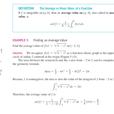
We begin with an arbitrary function ƒ defined on a closed interval [a,b]. Like the function pictured in Figure 5.8, ƒ may have negative as well as positive values. We subdi-vide the interval [a,b] into subintervals, not necessarily of equal widths (or lengths), and form sums in the same way as for the finite approximations in Section 5.1. To do so, we

choose points between aand band satisfying

To make the notation consistent, we denote aby and bby so that

The set

is called a partitionof [a,b].

The partition Pdivides [a,b] into nclosed subintervals

The first of these subintervals is the second is and the kth subinterval of Pis for [xk-1, xk] , kan integer between 1 and n.

[x1, x2] , [x0, x1] ,

[x0, x1], [x1, x2],Á, [xn-1, xn] .

P = 5x0, x1, x2,Á, xn-1, xn6

a = x0 6 x1 6 x2 6 Á 6 xn-1 6 xn = b.

xn,

x0

a 6 x1 6 x2 6 Á 6 xn-1 6 b. 5x1, x2, x3,Á, xn-16

n - 1 2>3

340

HISTORICALBIOGRAPHY Georg Friedrich

Bernhard Riemann (1826–1866)

x y

b a

y f(x)

(19)

The width of the first subinterval is denoted the width of the second is denoted and the width of the kth subinterval is If all n subintervals have equal width, then the common width is equal to

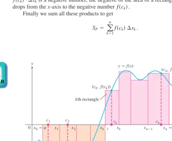
In each subinterval we select some point. The point chosen in the kth subinterval is called Then on each subinterval we stand a vertical rectangle that stretches from thex-axis to touch the curve at These rectangles can be above or below the x-axis, depending on whether is positive or negative, or on it if (Figure 5.9).

On each subinterval we form the product This product is positive,

nega-tive or zero, depending on the sign of When the product is

the area of a rectangle with height and width When the product is a negative number, the negative of the area of a rectangle of width that drops from the x-axis to the negative number

Finally we sum all these products to get

SP = a n

k=1

ƒsckd¢xk.

ƒsckd.

¢xk

ƒsckd

#

¢xk

ƒsckd 6 0 ,

¢xk.

ƒsckd

#

¢xk

ƒsckd 7 0 ,

ƒsckd.

ƒsckd

#

¢xk.

ƒsckd = 0

ƒsckd

sck, ƒsckdd.

ck.

[xk-1, xk]

x

• • • • • •

x₀a x₁ x₂ xk1 xk xn1 xnb

xn

xk

x1 x2

sb - ad>n.

¢x

¢xk = xk - xk-1.

¢x2, [x1, x2]

¢x1, [x0, x1]

x

• • • • • •

kth subinterval

x₀a x₁ x₂ x_k₁ x_k x_n₁ x_nb

341

x y

0

(c2, f(c2))

(c₁, f(c₁))

x₀ a x₁ x₂ xk1 xk xn1 xn b

ck cn

c₂ c₁

kth rectangle (ck, f(ck))

y f(x)

(cn, f(cn))

FIGURE 5.9 The rectangles approximate the region between the graph of the function and the x-axis.

(20)

The sum is called aRiemann sum forƒon the interval[a,b]. There are many such sums, depending on the partition Pwe choose, and the choices of the points in the subintervals. In Example 5, where the subintervals all had equal widths we could make them thinner by simply increasing their number n. When a partition has subintervals of varying widths, we can ensure they are all thin by controlling the width of a widest (longest) subinterval. We define the normof a partition P, written to be the largest of all the subinterval widths. If is a small number, then all of the subintervals in the parti-tion Phave a small width. Let’s look at an example of these ideas.

EXAMPLE 6 Partitioning a Closed Interval

The set is a partition of [0, 2]. There are five subintervals of P: [0, 0.2], [0.2, 0.6], [0.6, 1], [1, 1.5], and [1.5, 2]:

The lengths of the subintervals are and

The longest subinterval length is 0.5, so the norm of the partition is In this example, there are two subintervals of this length.

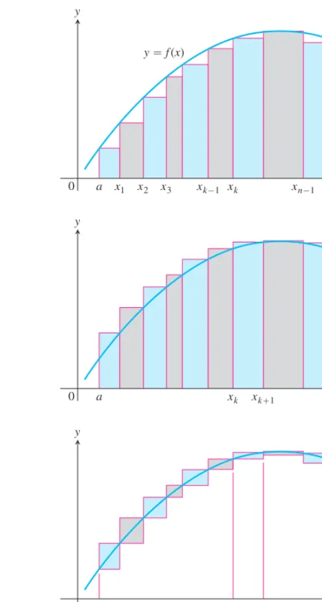
Any Riemann sum associated with a partition of a closed interval [a,b] defines rec-tangles that approximate the region between the graph of a continuous function ƒ and the x-axis. Partitions with norm approaching zero lead to collections of rectangles that approx-imate this region with increasing accuracy, as suggested by Figure 5.10. We will see in the next section that if the function ƒ is continuous over the closed interval [a,b], then no mat-ter how we choose the partition Pand the points in its subintervals to construct a Rie-mann sum, a single limiting value is approached as the subinterval widths, controlled by the norm of the partition, approach zero.

ck

7P7 = 0.5 .

¢x5 = 0.5 .

¢x1 = 0.2, ¢x2 = 0.4, ¢x3 = 0.4, ¢x4 = 0.5 , x

x1 x2 x3

0 0.2 0.6 1 1.5 2

x4 x5

P = {0, 0.2, 0.6, 1, 1.5, 2} 7P7

7P7,

¢x = 1>n, ck

SP

342

(a)

(b)

x

0 a b

y y

x

0 a b

yf(x)

(21)

342 EXERCISES 5.2

Sigma Notation

Write the sums in Exercises 1–6 without sigma notation. Then evalu-ate them.

1. 2.

3. 4.

5. 6.

7. Which of the following express in sigma notation?

a. b. c. _a

4

k= -1

2k+1 a

5

k=0

2k

a 6

k=1

2k-1

1+ 2+ 4 + 8 + 16 + 32

a 4

k=1s

-1dk_cos kp

a 3

k=1s

-1dk+1_sinp k

a 5

k=1 sin k

p

a 4

k=1 cos k

p

a 3

k=1 k - 1

k a

2

k=1

6k k + 1

8. Which of the following express in sigma notation?

a. b. c.

9. Which formula is not equivalent to the other two?

a. b. c.

10. Which formula is not equivalent to the other two?

a. b. c. _a

-1

k= -3 k2 a

3

k= -1 sk + 1d2 a

4

k=1 sk - 1d2

a 1

k= -1 s-1dk k + 2

a 2

k=0 s-1dk k + 1

a 4

k=2 s-1dk-1

k - 1

a 3

k= -2 s-1dk+1

2k+2

a 5

k=0 s-1dk

2k

a 6

k=1 s-2dk-1

(22)

Express the sums in Exercises 11–16 in sigma notation. The form of your answer will depend on your choice of the lower limit of summation.

11. 12.

13. 14.

15. 16.

Values of Finite Sums

17. Suppose that and Find the values of

a. b. c.

d. e.

18. Suppose that and Find the values of

a. b.

c. d.

Evaluate the sums in Exercises 19–28.

19. a. b. c.

Rectangles for Riemann Sums

In Exercises 29–32, graph each function ƒ(x) over the given interval. Partition the interval into four subintervals of equal length. Then add to your sketch the rectangles associated with the Riemann sum given that is the (a) left-hand endpoint, (b) right-hand endpoint, (c) midpoint of the kth subinterval. (Make a separate sketch for each set of rectangles.)

29. 30. 31. 32.

33. Find the norm of the partition

34. Find the norm of the partition

Limits of Upper Sums

For the functions in Exercises 35–40 find a formula for the upper sum obtained by dividing the interval [a,b] into nequal subintervals. Then take a limit of these sums as to calculate the area under the curve over [a,b].

35. over the interval [0, 1].

40. ƒsxd = 3x + 2x2over the interval [0, 1].

(23)

5.3 The Definite Integral

343 The Definite Integral

In Section 5.2 we investigated the limit of a finite sum for a function defined over a closed interval [a,b] using nsubintervals of equal width (or length), In this section we consider the limit of more general Riemann sums as the norm of the partitions of [a,b] approaches zero. For general Riemann sums the subintervals of the partitions need not have equal widths. The limiting process then leads to the definition of the definite integral of a function over a closed interval [a,b].

Limits of Riemann Sums

The definition of the definite integral is based on the idea that for certain functions, as the norm of the partitions of [a,b] approaches zero, the values of the corresponding Riemann

(24)

sums approach a limiting value I. What we mean by this converging idea is that a Riemann sum will be close to the number Iprovided that the norm of its partition is sufficiently small (so that all of its subintervals have thin enough widths). We introduce the symbol as a small positive number that specifies how close to Ithe Riemann sum must be, and the symbol as a second small positive number that specifies how small the norm of a parti-tion must be in order for that to happen. Here is a precise formulaparti-tion.

d

P

344

DEFINITION The Definite Integral as a Limit of Riemann Sums

Let ƒ(x) be a function defined on a closed interval [a,b]. We say that a number I is the definite integral of ƒover [a,b]and that Iis the limit of the Riemann sums if the following condition is satisfied:

Given any number there is a corresponding number such that

for every partition of [a,b] with and any choice of

in we have

`a

n

k=1

ƒsckd¢xk - I` 6 P.

[xk-1, xk] ,

ck

7P7 6 d

P = 5x0, x1,Á, xn6

d 7 0

P 7 0

gn

k=1ƒsckd¢xk

Leibniz introduced a notation for the definite integral that captures its construction as a limit of Riemann sums. He envisioned the finite sums becoming an infi-nite sum of function values ƒ(x) multiplied by “infiinfi-nitesimal” subinterval widths dx. The sum symbol is replaced in the limit by the integral symbol whose origin is in the letter “S.” The function values are replaced by a continuous selection of function val-ues ƒ(x). The subinterval widths become the differential dx. It is as if we are summing all products of the form as xgoes from ato b. While this notation captures the process of constructing an integral, it is Riemann’s definition that gives a precise meaning to the definite integral.

Notation and Existence of the Definite Integral

The symbol for the number Iin the definition of the definite integral is

which is read as “the integral from ato bof ƒ of xdee x” or sometimes as “the integral from ato bof ƒ of xwith respect to x.” The component parts in the integral symbol also have names:

⌠



⌡

      

The function is the integrand.

x is the variable of integration.

When you find the value of the integral, you have evaluated the integral. Upper limit of integration

Integral sign

Lower limit of integration

Integral of f from a to b

a

b

f

(x) dx

L

b

a

ƒsxddx ƒsxd

#

dx

¢xk

ƒsckd

1,

a

gn

(25)

When the definition is satisfied, we say the Riemann sums of ƒ on [a,b] convergeto the definite integral and that ƒ is integrableover [a,b]. We have many choices for a partition Pwith norm going to zero, and many choices of points for each partition. The definite integral exists when we always get the same limit I, no matter what choices are made. When the limit exists we write it as the definite integral

When each partition has nequal subintervals, each of width we will also write

The limit is always taken as the norm of the partitions approaches zero and the number of subintervals goes to infinity.

The value of the definite integral of a function over any particular interval depends on the function, not on the letter we choose to represent its independent variable. If we decide to use tor uinstead of x, we simply write the integral as

No matter how we write the integral, it is still the same number, defined as a limit of Rie-mann sums. Since it does not matter what letter we use, the variable of integration is called a dummy variable.

Since there are so many choices to be made in taking a limit of Riemann sums, it might seem difficult to show that such a limit exists. It turns out, however, that no matter what choices are made, the Riemann sums associated with a continuousfunction converge to the same limit.

L

b

a

ƒstd dt or L

b

a

ƒsud du instead of L

b

a

ƒsxd dx. lim

n:q a

n

k=1

ƒsckd¢x = I =

L

b

a

ƒsxddx.

¢x = sb - ad>n, lim

ƒ ƒPƒ ƒ:0a

n

k=1

ƒsckd¢xk = I =

L

b

a

ƒsxddx.

ck

I = ₁_abƒsxd dx

345

THEOREM 1 The Existence of Definite Integrals

A continuous function is integrable. That is, if a function ƒ is continuous on an interval [a,b], then its definite integral over [a,b] exists.

By the Extreme Value Theorem (Theorem 1, Section 4.1), when ƒ is continuous we can choose so that gives the maximum value of ƒ on giving an upper sum. We can choose to give the minimum value of ƒ on giving a lower sum. We can pick to be the midpoint of the rightmost point or a random point. We can take the partitions of equal or varying widths. In each case we get the same limit

for as The idea behind Theorem 1 is that a Riemann sum

asso-ciated with a partition is no more than the upper sum of that partition and no less than the lower sum. The upper and lower sums converge to the same value when All other Riemann sums lie between the upper and lower sums and have the same limit. A proof of Theorem 1 involves a careful analysis of functions, partitions, and limits along this line of thinking and is left to a more advanced text. An indication of this proof is given in Exercises 80 and 81.

7P7_:0 . 7P7_:0 .

gn

k=1ƒsckd¢xk

xk,

[xk-1, xk] ,

ck

[xk-1, xk] ,

ck

[xk-1, xk] ,

ƒsckd

(26)

Theorem 1 says nothing about how to calculatedefinite integrals. A method of calcu-lation will be developed in Section 5.4, through a connection to the process of taking anti-derivatives.

Integrable and Nonintegrable Functions

Theorem 1 tells us that functions continuous over the interval [a,b] are integrable there. Functions that are not continuous may or may not be integrable. Discontinuous functions that are integrable include those that are increasing on [a,b] (Exercise 77), and the piecewise-continuous functionsdefined in the Additional Exercises at the end of this chap-ter. (The latter are continuous except at a finite number of points in [a,b].) For integrabil-ity to fail, a function needs to be sufficiently discontinuous so that the region between its graph and the x-axis cannot be approximated well by increasingly thin rectangles. Here is an example of a function that is not integrable.

EXAMPLE 1 A Nonintegrable Function on [0, 1]

The function

has no Riemann integral over [0, 1]. Underlying this is the fact that between any two num-bers there is both a rational number and an irrational number. Thus the function jumps up and down too erratically over [0, 1] to allow the region beneath its graph and above the x-axis to be approximated by rectangles, no matter how thin they are. We show, in fact, that upper sum approximations and lower sum approximations converge to different limiting values.

If we pick a partition Pof [0, 1] and choose to be the maximum value for ƒ on then the corresponding Riemann sum is

since each subinterval contains a rational number where Note that the lengths of the intervals in the partition sum to 1, So each such Riemann sum equals 1, and a limit of Riemann sums using these choices equals 1.

On the other hand, if we pick to be the minimum value for ƒ on then the Riemann sum is

since each subinterval contains an irrational number where The limit of Riemann sums using these choices equals zero. Since the limit depends on the choices of the function ƒ is not integrable.

Properties of Definite Integrals

In defining as a limit of sums we moved from left to right

across the interval [a,b]. What would happen if we instead move right to left, starting with and ending at Each in the Riemann sum would change its sign, with now negative instead of positive. With the same choices of in each subinter-val, the sign of any Riemann sum would change, as would the sign of the limit, the integral

ck

xk - xk-1

¢xk

xn = a.

x0 = b

gn

k=1ƒsckd¢xk,

1abƒsxd dx

ck,

ƒsckd = 0 .

ck

[xk-1, xk]

L = _a

n

k=1

ƒsckd¢xk = a n

k=1

s0d¢xk = 0 ,

[xk-1, xk] ,

ck

gn

k=1¢xk = 1 .

ƒsckd = 1 .

[xk-1, xk]

U = _a

n

k=1

ƒsckd¢xk = a n

k=1

s1d¢xk = 1 ,

[xk-1, xk]

ck

ƒsxd = e1, if x is rational

0, if x is irrational

(27)

Since we have not previously given a meaning to integrating backward, we are led to define

Another extension of the integral is to an interval of zero width, when Since is zero when the interval width , we define

Theorem 2 states seven properties of integrals, given as rules that they satisfy, includ-ing the two above. These rules become very useful in the process of computinclud-ing integrals. We will refer to them repeatedly to simplify our calculations.

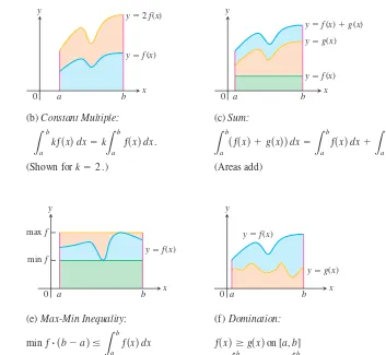
Rules 2 through 7 have geometric interpretations, shown in Figure 5.11. The graphs in these figures are of positive functions, but the rules apply to general integrable functions.

L

347

THEOREM 2

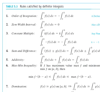
When ƒ andgare integrable, the definite integral satisfies Rules 1 to 7 in Table 5.3.

TABLE 5.3 Rules satisfied by definite integrals

1. Order of Integration: A Definition

2. Zero Width Interval: Also a Definition

3. Constant Multiple: Any Number k

4. Sum and Difference:

5. Additivity:

(28)

While Rules 1 and 2 are definitions, Rules 3 to 7 of Table 5.3 must be proved. The proofs are based on the definition of the definite integral as a limit of Riemann sums. The following is a proof of one of these rules. Similar proofs can be given to verify the other properties in Table 5.3.

Proof of Rule 6 Rule 6 says that the integral of ƒ over [a,b] is never smaller than the minimum value of ƒ times the length of the interval and never larger than the maximum value of ƒ times the length of the interval. The reason is that for every partition of [a,b] and for every choice of the points

Constant Multiple Rule

= max ƒ

#

sb - ad.

348

x

(a) Zero Width Interval:

(The area over a point is 0.)

L

a

ƒsxddx = 0 .

(b) Constant Multiple:

(Shown for k = 2 .)

(d) Additivity for definite integrals:

L

(e) Max-Min Inequality:

(29)

In short, all Riemann sums for ƒ on [a,b] satisfy the inequality

Hence their limit, the integral, does too.

EXAMPLE 2 Using the Rules for Definite Integrals

Suppose that

Then

1. Rule 1

2. Rules 3 and 4

3. Rule 5

EXAMPLE 3 Finding Bounds for an Integral

Show that the value of is less than .

Solution The Max-Min Inequality for definite integrals (Rule 6) says that

is a lower boundfor the value of and that is an upper bound.

The maximum value of on [0, 1] is so

Since is bounded from above by (which is 1.414 ), the integral is less than .

Area Under the Graph of a Nonnegative Function

We now make precise the notion of the area of a region with curved boundary, capturing the idea of approximating a region by increasingly many rectangles. The area under the graph of a nonnegative continuous function is defined to be a definite integral.

3>2

Á

22

10121 + cosx dx

L 1

0

21 + cosx dx … 22

#

s1 - 0d = 22 . 21 + 1 = 22 , 21 + cosx

max ƒ

#

sb - ad

1abƒsxd dx

min ƒ

#

sb - ad 3>2

10121 + cosx dx

L 4

-1

ƒsxd dx =

L 1

-1

ƒsxd dx +

L 4

1

ƒsxd dx = 5 + s-2d = 3

= 2s5d + 3s7d = 31 L

1

-1

[2ƒsxd + 3hsxd] dx = 2 L

1

-1

ƒsxd dx + 3 L

1

-1 hsxd dx L

1

4

ƒsxd dx =

-L 4

1

ƒsxd dx = -s-2d = 2 L

1

-1

ƒsxd dx = 5, L

4

1

ƒsxd dx = -2, L

1

-1

hsxd dx = 7 . min ƒ

#

sb - ad … _a

n

k=1

ƒsckd¢xk … max ƒ

#

sb - ad.

349

DEFINITION Area Under a Curve as a Definite Integral

If is nonnegative and integrable over a closed interval [a,b], then the area under the curve over [a,b] is the integral of ƒ from ato b,

A =

L

b

a

ƒsxd dx.

y = ƒsxd

(30)

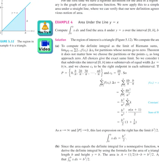
For the first time we have a rigorous definition for the area of a region whose bound-ary is the graph of any continuous function. We now apply this to a simple example, the area under a straight line, where we can verify that our new definition agrees with our pre-vious notion of area.

EXAMPLE 4 Area Under the Line

Compute and find the area Aunder over the interval [0,b],

Solution The region of interest is a triangle (Figure 5.12). We compute the area in two ways. (a) To compute the definite integral as the limit of Riemann sums, we calculate for partitions whose norms go to zero. Theorem 1 tells us that it does not matter how we choose the partitions or the points as long as the norms approach zero. All choices give the exact same limit. So we consider the partition P that subdivides the interval [0,b] intonsubintervals of equal width

and we choose to be the right endpoint in each subinterval. The partition is and So

Constant Multiple Rule

Sum of First nIntegers

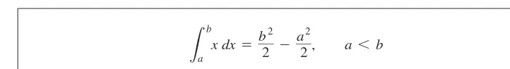
As and this last expression on the right has the limit Therefore,

(b) Since the area equals the definite integral for a nonnegative function, we can quickly derive the definite integral by using the formula for the area of a triangle having base

length b and height The area is Again we have

that

Example 4 can be generalized to integrate over any closed interval

Rule 5

350

x

(31)

In conclusion, we have the following rule for integrating f(x) = x:

351

(1)

L

b

a

x dx = b2

2

-a2

2, a 6 b

This computation gives the area of a trapezoid (Figure 5.13). Equation (1) remains valid when aand bare negative. When the definite integral value is a negative number, the negative of the area of a trapezoid dropping down to the line below the x-axis. When and Equation (1) is still valid and the definite inte-gral gives the difference between two areas, the area under the graph and above [0,b] minus the area below [a, 0] and over the graph.

The following results can also be established using a Riemann sum calculation similar to that in Example 4 (Exercises 75 and 76).

b 7 0 , a 6 0

y = x sb2 - a2d>2 a 6 b 6 0 ,

(2)

(3)

L

b

a

x2 dx = b3

3

-a3

3, a 6 b

L

b

a

c dx = csb - ad, c any constant x

y

0

a

a b

b a

b

ba yx

FIGURE 5.13 The area of this trapezoidal region is

A = sb2 - a2d>2 .

Average Value of a Continuous Function Revisited

In Section 5.1 we introduced informally the average value of a nonnegative continuous function ƒ over an interval [a,b], leading us to define this average as the area under the graph of divided by In integral notation we write this as

We can use this formula to give a precise definition of the average value of any continuous (or integrable) function, whether positive, negative or both.

Alternately, we can use the following reasoning. We start with the idea from arith-metic that the average of nnumbers is their sum divided by n. A continuous function ƒ on [a,b] may have infinitely many values, but we can still sample them in an orderly way. We divide [a,b] into nsubintervals of equal width and evaluate ƒ at a point

in each (Figure 5.14). The average of the nsampled values is

= 1

b - a a

n

k=1

ƒsckd¢x

¢x= b-_na, so 1_n = ¢x b-a = ¢x

b- a a

n

k=1 ƒsckd

ƒsc1d + ƒsc2d + Á + ƒscnd

n = 1na