Method Validation in Pharmaceutical Analysis A Guide to Best Practice

(1)

Method Validation

in Pharmaceutical Analysis

Edited by

J. Ermer and J. H. McB. Miller

(2)

Related Titles from Wiley-VCH:

M. S. Lee

LC/MS Applications in Drug Development

2002

ISBN: 0-471-40520-5

M. Stoeppler, W. R. Wolf, P. J. Jenks (Eds.)

Reference Materials for Chemical Analysis

Certification, Availability, and Proper Usage

2001

ISBN: 3-527-30162-3

J. M. Miller, J. B. Crowther (Eds.)

Analytical Chemistry in a GMP Environment

A Practical Guide

2000

(3)

Method Validation in Pharmaceutical Analysis

A Guide to Best Practice

Edited by

(4)

Dr. Joachim Ermer sanofi-aventis Industriepark Hchst Build. G875 65926 Frankfurt Germany

Dr. John H. McB. Miller

European Directorate for the Quality of Medicines (EDQM)

16, Rue Auguste Himly 67000 Strasbourg France

editors, authors, and publisher do not warrant the information contained therein to be free of errors. Readers are advised to keep in mind that statements, data, illustrations, procedural details or other items may inadvertently be inaccurate.

Library of Congress Card No. applied for

British Library Cataloguing-in-Publication Data A catalogue record for this book is available from the British Library.

Bibliographic information published by Die Deutsche Bibliothek

Die Deutsche Bibliothek lists this publication in the Deutsche Nationalbibliografie; detailed bibliographic data is available in the Internet at <http://dnb.ddb.de>.

2005 WILEY-VCH Verlag GmbH & Co. KGaA, Weinheim

All rights reserved (including those of translation into other languages). No part of this book may be reproduced in any form – by photoprinting, micro-film, or any other means – nor transmitted or trans-lated into machine language without written permis-sion from the publishers. Registered names, trade-marks, etc. used in this book, even when not specifically marked as such, are not to be considered unprotected by law.

Printed in the Federal Republic of Germany. Printed on acid-free paper.

Typesetting Khn & Weyh, Satz und Medien, Freiburg

Printing betz-druck GmbH, Darmstadt Bookbinding Litges & Dopf Buchbinderei GmbH, Heppenheim

(5)

A number of articles and guidelines already exist dealing with the validation of ana-lytical methods. However, the editors consider that none of the texts completely cov-ers all aspects pertinent to analytical validation for, in particular, methods in phar-maceutical analysis. The editors have attempted, with the authors of the relevant chapters, to bring all these elements together in one book that will be useful to both analysts in the pharmaceutical industry (and beyond) as well as to assessors at the registration authorities for medicines.

Methods used in pharmaceutical analysis must be sufficiently accurate, specific, sensitive and precise to conform to the regulatory requirements as set out in the relevant guidelines of "The International Conference of Technical Requirements for the Registration of Pharmaceutical for Human Use " (ICH), which are applied by the licensing authorities and by some pharmacopoeias. The chapters in Part I deal specifically with the fundamentals of the different validation parameters, giving spe-cial emphasis to practical examples and recommendations. It is not intended to replace statistical textbooks but the editors have attempted to provide sufficient back-ground information, illustrated by practical examples to aid the reader in under-standing and choosing the relevant parameters and acceptance criteria to be consid-ered for the application of any one analytical procedure to a particular purpose.

Contributions to Part II of this book deal with the life-cycle approach to validation starting with the qualification of equipment employed, the adaptation of ICH guide-lines to the early stages of drug development, the relation between analytical vari-ability and specification acceptance criteria, the continual assessment of the perfor-mance of the methods when in regular use, the transfer of analytical procedures, and out-of-specification results. There are also chapters dealing with the validation of pharmacopoeial methods and future perspectives for validation.

December 2004 John H. McB. Miller

Joachim Ermer

V

Preface

(6)

Preface V

List of Contributors XIII

Part I Fundamentals of Validation in Pharmaceutical Analysis 1

1 Analytical Validation within the Pharmaceutical Environment 3

Joachim Ermer

1.1 Regulatory Requirements 4

1.2 Integrated and Continuous Validation 5

1.3 General Planning and Design of Validation Studies 7

1.3.1 Always Look on the Routine’ Side of Validation 8

1.4 Evaluation and Acceptance Criteria 9

1.4.1 What does Suitability Mean? 9

1.4.2 Statistical Tests 12

1.5 Key Points 14

2 Performance Parameters, Calculations and Tests 21

2.1 Precision 21

Joachim Ermer

2.1.1 Parameters Describing the Distribution of Analytical Data 22

2.1.2 Precision Levels 30

2.1.3 Acceptable Ranges for Precisions 35

2.1.4 Sources to Obtain and Supplement Precisions 49

2.1.5 Key Points 51

2.2 Specificity 52

Joachim Ermer

2.2.1 Demonstration of Specificity by Accuracy 55

2.2.2 Chromatographic Resolution 55

2.2.3 Peak Purity (Co-elution) 57

2.2.4 Key Points 62

List of Contributors

(13)

Prof. Hermann Wtzig

Technical University Braunschweig Institut fr Pharmazeutische Chemie Beethovenstr. 55

38106 Braunschweig Germany

(14)

Part I:

Fundamentals of Validation in Pharmaceutical Analysis

(15)

3

Validation is, of course, a basic requirement to ensure quality and reliability of the results for all analytical applications [8]. However, in comparison with analytical chemistry, in pharmaceutical analysis, some special aspects and conditions exist that need to be taken into consideration. For example, the analytical procedures (apart from pharmacopoeial monographs) are often in-house developments and applications. Therefore, the degree of knowledge and expertise is initially much larg-er compared with standard methods. The same can be assumed for the samples analysed. The matrix (placebo) in pharmaceutical analysis is usually constant and well known and the ranges where the sample under analysis can be expected are usually well defined and not very large. Evaluation (of batches, stability investiga-tions, etc.) is based on the results of various procedures or control tests, thus their performances can complement each other. Acceptance limits of the specification are fixed values, often based on tradition, as in the case of assay of an active ingredient, or they may be based on specific toxicological studies, which take large safety factors into account, as for impurities. Last, but not least, validation in pharmaceutical anal-ysis has its own regulations. These few – by far from exhaustive – remarks should make it obvious that these special considerations will have an impact on the way validation in pharmaceutical analysis is performed.

The first part of this book focusses on the fundamentals of validation in

pharma-ceutical analysis, the environmental’ framework as well as the implications for

experimental design and suitable calculations. Of course, the basic principles of vali-dation are the same for any analytical procedure, regardless of its field of applica-tion. However, the discussions and recommendations focus on pharmaceutical applications, so the reader needs to adjust these to suit his or her purpose, if differ-ent. Nevertheless – as validation should never be regarded as simply working through a checklist – this is also required in the case of pharmaceutical analysis, but perhaps to a lesser extent, compared with other areas of application.

1

Analytical Validation within the Pharmaceutical Environment

Joachim Ermer

(16)

1.1

Regulatory Requirements

“The object of validation of an analytical procedure is to demonstrate that it is suitable for its intended purpose” [1a], determined by means of well-documented experimental studies. Accuracy and reliability of the analytical results is crucial for ensuring qual-ity, safety and efficacy of pharmaceuticals. For this reason, regulatory requirements have been published for many years [1–7].

The International Conference on the Harmonisation of Technical Requirements for the Registration of Pharmaceuticals for Human Use (ICH) was initiated in 1990, as a forum for a constructive dialogue between regulatory authorities and industry, in order to harmonise the submission requirements for new pharmaceuticals be-tween Europe, the United States of America and Japan. One of the first topics within the Quality section was analytical validation and the ICH was very helpful in harmo-nising terms and definitions [1a] as well as determining the basic requirements [1b]. Of course, due to the nature of the harmonisation process, there are some compro-mises and inconsistencies. In Table 1-1, the required validation characteristics for the various types of analytical procedures are shown.

Table 1-1: Validation characteristics normally evaluated for the different types of test procedures [1a] and the minimum number of determinations required [1b]

Analytical procedure

Validation characteristic

Minimum number

Identity Impurities Assay1

Quantitative Limit

1. Specificity2 _{Not applicable} _Yes _Yes _Yes _Yes

2. Linearity 5 No Yes No Yes

3. Range Not applicable No Yes No Yes

4. Accuracy 9 (e.g. 3 3) No Yes No Yes

5. Precision

Repeatability 6 or 9 (e.g. 3 3) No Yes No Yes

Intermediate precision/ Reproducibility3

(2 series)4 No Yes No Yes

6. Detection limit Approach dependent No No5 Yes No

7. Quantitation limit No Yes No No

Yes / No normally evaluated / not evaluated 1 including dissolution, content/potency

2 lack of specificity of one analytical procedure could be compensated by other supporting analytical procedure(s)

(17)

1.2 Integrated and Continuous Validation

Two guidelines on validation were issued by the US Food and Drug Administration (FDA), one for the applicant [2], the other for inspectors and reviewers [3]. The first one is also intended to ensure that the analytical procedure can be applied in an FDA laboratory and therefore requires a detailed description of the procedure, reference materials, as well as a discussion of the potential impurities, etc. The second guide-line focuses on reversed-phase chromatography and provides a lot of details with regard to critical methodological issues, as well as some indication of acceptability of results. A revised draft of the first guideline was published in 2000 [4]. According to

the title “Analytical procedures and methods validation”, it also includes the content and

format of the analytical procedures, the requirements for reference standards and var-ious types of analytical technique. Therefore, this guidance is more comprehensive

than the ICH Guidelines, but is rather too focussed on providinginstrument output/

raw data’. As this is an inspection and documentation issue, it should be separated from the validation. A very detailed discussion is provided in the Canadian guideline [7] with respect to requirements and particularly acceptance criteria. Although this allows some orientation, the given acceptance criteria were sometimes rather too ambiguous, for example, the intermediate precision / reproducibility of less than 1% for drug substances (see Section 2.1.3.2 and Fig. 2.1-12).

So why is it still important to discuss validation?

First of all, the ICH guidelines should be regarded as the basis and philosophical background to analytical validation, not as a checklist.“It is the responsibility of the applicant to choose the validation procedure and protocol most suitable for their product” [1b]. It will be shown in the next sections that suitability is strongly connected with the requirements and design of the given analytical procedure. As this obviously var-ies, at least with the type of procedure, it must be reflected in the analytical valida-tion. This includes the identification of the performance parameters relevant for the given procedure, the definition of appropriate acceptance criteria and the appropri-ate design of the validation studies. In order to achieve this, the analyst must be aware of the fundamental meaning of these performance parameters, as well as the calculations and tests and their relationship to the specific application. The former is discussed in detail in Chapter 2, the latter in the following sections. A lack of knowledge or (perhaps) a wrong understanding of efficiency’ will lead to validation results that address the real performance of the analytical procedure only partly or insufficiently. This is, at the very least a waste of work, because the results are mean-ingless. Unfortunately, this can also be found rather too frequently in publications, although to a varying extent for the different validation characteristics. Such com-mon insufficiencies are discussed in the respective sections of Chapter 2.

1.2

Integrated and Continuous Validation

Validation should not be regarded as a singular activity [4], but should always be understood with respect to the life cycle of the analytical procedure. Starting with the method development or optimisation, the performance of the analytical

(18)

dure should be matched to the requirements in aniterative process. Some validation characteristics, such as specificity (selective separation) or robustness, are more important in this stage (see Section 2.7). However, this depends on the type of pro-cedure. In the case of a complex sample preparation, or cleaning methods (see Sec-tion 2.3.4), precision and accuracy may play an important role in the optimisaSec-tion process. One should also be aware that the validation requested for submission, i. e.

a demonstration of thegeneralsuitability of the respective analytical procedure – can

only be considered as a basis. The user of any method has to guarantee that it will stay consistently in a validated status, also referred to as the life-cycle concept of ana-lytical validation [9]. In this process, an increasing amount of information can be compiled.

This does not necessarily mean that additional work always needs to be done. Dur-ing the actual application of the methods, a lot of data is generated, but often left

unused(data graveyard’). In order to make rational and efficient use of these data,

they must be transformed to information (i.e., processed and condensed into perfor-mance parameters). When enough reliable information is compiled, it can be further processed to gain knowledge that eventually enables us to achieve a better under-standing and control of the analytical procedure (see also Section 2.1.4 and Chapter 9). The whole process is well known as aninformation pyramid’(Fig. 1-1). This knowl-edge can also be used to improve analytical procedures, for example, by changing from the traditional daily’ calibration in an LC assay to a quantitation using predeter-mined’ calibration parameters (comparable to a specific absorbance in spectropho-tometry), with advantages both in efficiency and reduced analytical variability [10].

Transfersof analytical procedures to another site of the company or to a contract laboratory – quite common nowadays – often result in a challenging robustness test, especially if not appropriately addressed in the validation. Acceptance criteria for a successful transfer may be derived from the validation itself, or from the same prin-ciples as for calculations and tests in validation, because here the performance of the analytical procedure is also addressed (see Chapter 7). On the other hand, com-parative studies will provide quite reliable performance data of the analytical proce-dure (see Section 2.1.3.2).

Besides this horizontal’ integration, analytical validation also needs to be included in the whole system ofAnalytical Quality Assurance(AQA) [8], i.e., vertical’ integration. This involves all (internal and external) measures which will ensure the quality and reliability of the analytical data, such as an equipment qualification program (see Chapter 4), appropriate system suitability tests (see Section 2.8), good documentation and review practices, operator training, control charts (see Chapter 9), etc.

Information

Data

Control

Knowledge

(19)

1.3 General Planning and Design of Validation Studies

1.3

General Planning and Design of Validation Studies

Performance is strongly connected with the requirements and design of the given analytical procedure (see Section 1.4.1). As this obviously varies, it must be reflected in the planning and design of the analytical validation. Consequently, a checklist approach is not appropriate. In order to ensure thorough planning, i.e., to identify the relevant performance parameters, to define appropriate acceptance criteria and

then to design the studies accordingly, validation protocolsshould be prepared. In

addition to thisgood science’ reason, protocols can also be regarded as a general

GMP requirement and are common practice also the in case of process validation, cleaning validation, equipment qualification, transfer, etc.

The analyst may be faced with the problem of the iterative nature of the method development / validation process. However, here one may distinguish between per-formance parameters (and the corresponding validation characteristics) of the final analytical procedure and those obtained or derived from different method condi-tions, such as specificity and robustness. The former can be addressed (before start-ing the experimental studies, followstart-ing usual practice) in the protocol, the latter can be referred to in the validation report and/or protocol (see Chapter 5).

Of course, theextent and depthof the validation studies, as well as acceptance cri-teria, should be defined in relation to the required performance (importance’) and the environment’ of the respective analytical procedure, such as the stages of devel-opment (see Chapter 5), or the stages of manufacturing / synthesis. Important or critical procedures (within the context of validation) can be expected to have tighter specification limits. In these cases, such as the assay of active or of critical impuri-ties, it is recommended to address the validation characteristicsseparately(for exam-ple, precision with authentic samples and accuracy with spiked samples),in order to increase the power of the results. In other cases, such as the determination of other ingredients or of impurities or water sufficiently below specification limits, several validation characteristics, for example, precision, linearity, and accuracy (quantita-tion) limit in dependence on the range, see Section 2.6.4) can be investigated simul-taneously, using the same spiked samples.

The ICH Guidelines [1a,b] are mainly focused on chromatographic procedures, as can be seen in the methodology guideline [1b]. Therefore, they should be regarded more as a guide to thephilosophy of validation– i.e., used to identify relevant perfor-mance parameters of the given analytical procedure – than as a holy grail’. If the special conditions or techniques are not covered in the ICH guideline, the validation approach must then be adapted accordingly (see Chapter 11). The FDA Guidance [4], and the Technical Guide of the European Pharmacopoeia (EP) [11], as well as Chapter 8 also provide details for specific analytical techniques.

(20)

1.3.1

Always Look on the Routine’ Side of Validation

Curiously, one aspect often neglected during validation is its primary objective, i.e.,

to obtain the realperformance of the routine applicationof the analytical procedure. As

far as possible, all steps of the procedure should be performed as described in the control test. Of course, this cannot always achieved, but at least the analyst should always be aware of such differences, in order to evaluate the results properly.

What does this mean in practice?

For example, precision should preferably be investigated usingauthenticsamples,

because only in this case is the sample preparation identical to the routine applica-tion. It is also important to apply the intended calibration mode exactly as described in the analytical procedure. Sometimes the latter is not even mentioned in the litera-ture. Precision is reported only from repeated injections of the same solution, ignor-ing the whole sample preparation. This is certainly not representative for the (rou-tine) variability of the analytical procedure (see Section 2.1.2). Investigating pure so-lutions is usually of very limited practical use, for example, in the case of cleaning methods (see Section 2.3.4) or quantitation limit (see Section 2.6), or may even lead to wrong conclusions, as the following examples will show.

The minor (impurity) enantiomer of a chiral active ingredient was analysed by

chiral LC using an immobilised enzyme column (Chiral-CBH 5mm, 100 4 mm,

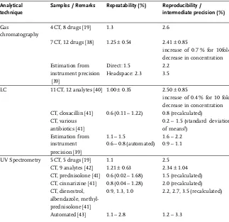
ChromTech). The quantitation should be carried out by area normalisation (100%-method, 100%-standard), which would require a linear response function and a neg-ligible intercept for both active and impurity enantiomer (see also Section 2.4.1). The experimental linearity investigation of dilutions of the active, revealed a clear devia-tion from a linear response funcdevia-tion (Fig. 1-2). However, when the design was adjusted to simulate the conditions of the routine application, i.e., spiking the impu-rity enantiomer to the nominal concentration of the active, an acceptable linear rela-tionship was found. Although a slight trend remained in the results, the recoveries between 99 and 105% can be regarded as acceptable for the intended purpose. A pos-sible explanation for such behaviour might be that the interaction between the enan-tiomers and the binding centres of the immobilised enzyme (cellobiohydrolase, hydrolysing crystalline cellulose) is concentration dependent. Maintaining the nom-inal test concentration in the case of the spiked samples, the sum of both enantio-mers is kept constant and consequently so are the conditions for interactions. In this case, the linearity of the active enantiomer cannot be investigated separately and the validity of the 100% method must be demonstrated by obtaining an acceptable recovery.

Stress samples

(21)

degra-1.4 Evaluation and Acceptance Criteria

dants “likely to be present” [1b], rather than alast resort’. However, it is also

reason-able to allow for some buffer’ [12].

Sometimes, applying artificial conditions cannot be avoided, in order to approach validation parameters, as in recovery investigations (see Section 2.3.2) or in dissolu-tion, where no homogeneous samples are available. In the latter case, the assay part of the analytical procedure may be investigated separately. However, possible influ-ences on the results due to the different application conditions need to be taken into account in the evaluation process as well as in the definition of acceptance criteria.

1.4

Evaluation and Acceptance Criteria

1.4.1

What does Suitability Mean?

The suitability of an analytical procedure is primarily determined by the require-ments of the given test item, and secondly by its design (which is normally more flexible). Usually, the (minimum) requirements are defined by the acceptance limits of the specification (often termed traditionally as specification limits’, but according to ICH [1e], the term specification’ defines a“list of tests, references to analytical

proce-9

0 20 40 60 80 100 120 140 160 180 200

0% 5% 10% 15% 20%

Analyte (%)

P

e

ak ar

e

a

(

u

ni

ts

)

Diluted

Spiked

Regression, diluted

Regression, spiked

(22)

dures, and appropriate acceptance criteria”). For some applications, the requirements are explicitly defined in the ICH Guidelines. For example, the reporting level for unknown degradants in drug products is set to 0.1% and 0.05% for a maximum daily intake of less and more than 1 g active, respectively [1d] (Table 2.6-1). In the case of cleaning validation, the maximum acceptable amount of cross-contamination can be calculated based on the batch sizes and doses of the previous and subsequent prod-uct, the toxicological or pharmacological activity and/or the safety factors, and the so called specific residual cleaning limit (SRCL) [13]. Consequently, the corresponding test procedure must be able to quantify impurities or residual substance at this con-centration with an appropriate level of precision and accuracy (see Section 2.3.4).

With respect to stability studies, the analytical variability must be appropriate to detect a (not acceptable) change in the tested property of the batch. This is illustrated in Figure 1-3 for determination of the content of active ingredient. The intrinsic deg-radation of 1.0% within 36 months can be reliably detected by an assay with a true variability of 0.5% (Fig. 1-3A), but not by one with 2.0% variability (Fig. 1-3B). Gen-erally, acceptance limits of the specification (SL) have to enclose (at least) both the analytical and the manufacturing variability (see Chapter 6). Rearranging the equa-tion describing this relaequa-tionship (Eq. 6-12), the maximum permitted analytical vari-ability can be calculated from the acceptance limits of the specification (Eq.1-1).

RSDmaxð%_{Þ ¼}jðBL SLÞj

ffiffiffiffiffiffiffiffiffiffi nassay p

tðP;dfÞ (1-1)

SL: Acceptance limits of the specification for active (% label claim).

BL: Basic limits, 100% – maximum variation of the manufacturing process

(in %). In case of shelf-life limits, the lower basic limit will additionally include the maximum acceptable decrease in the content.

94% 95% 96% 97% 98% 99% 100% 101%

0 10 20 30 40

Storage interval (months)

Content (%)

A

94% 95% 96% 97% 98% 99% 100% 101%

0 10 20 30 40

Storage interval (months)

B

(23)

1.4 Evaluation and Acceptance Criteria

nassay: Number of repeated, independent determinations in routine analyses, insofar as the mean is the reportable result, i.e., is compared to the accep-tance limits. If each individual determination is defined as the reportable

result,n=1 has to be used.

t(P,df): Studentt-factor for the defined level of statistical confidence (usually 95%) and the degrees of freedom in the respective precision study.

The same basic considerations of the relationship between content limits and an-alytical variability [14] were applied to the system precision (injection repeatability) requirements of the EP [15] (see Section 2.8.3.8). The method capability index (see Section 10.5, Eq. 10-5) is based on similar considerations. However, here the normal distribution is used to describe the range required for the analytical variability (see Section 2.1.1). Consequently, the method capability index must be applied to single determinations (or to means if the standard deviation of means is used) and requires a very reliable standard deviation, whereas Eq.(1-1) can take a variable num-ber of determinations directly into account, as well as the reliability of the

experi-mental standard deviation (by means of the Studentt-factor).

Of course, the precision acceptance limit thus obtained will be the minimum requirement. If a tighter control is needed, or if a lower variability is expected for the given type of method (analytical state of the art, see Section 2.1.3), the acceptance limits should be adjusted. A further adjustment may be required if there is a larger difference between repeatability and intermediate precision, i.e., if there is a larger inter-serial contribution (Eq. (2.1-10), Section 2.1.3.2). In such a case, an increased number of determinations in the assay will only reduce the repeatability variance,

but not the variance between the series (s2g). Therefore, the termpffiffiffiffiffiffiffiffiffiffinassay must be

transferred to the left-hand side of Eq. (1-1) and RSDmax(%) rearranged to

ffiffiffiffiffiffiffiffiffiffiffiffiffiffiffiffiffiffi s2

gþ s2

r

nassay

r

. This term corresponds to the standard deviation of the means from the

routine assay determinations.

Many other performance parameters are linked with the analytical variability. Therefore, once an acceptable precision is defined, it can serve as an orientation for other acceptance criteria (for details, see Table 1-2 and Sections 2.1–2.6). As far as

possible, normalised (percentage) parametersshould be defined as validation

accep-tance limits, because they can be compared across methods and therefore more eas-ily drawn from previous experience.

As can be seen from Eq. (1-1), the number of determinations also influences the acceptable performance, as well as the intended calibration mode (see Section 2.4). In principle, the analyst is rather flexible in his/her decision, provided that the minimum requirements are fulfilled. Often, the design of the calibration is more influenced by tradition or technical restrictions (for example the capabilities of the acquisition

soft-ware) than by scientific reasons. Sometimes acheck standard’ is applied, i.e., the

standard prepared and used for calibration is verified by a second standard prepara-tion, the response of which needs to be within an acceptable range of the first one (e.g.–1.0%). This approach is not optimal. If the check standard’ is only used for verification, 50% of the available data are ignored. Increasing the number of

(24)

nations improves the reliability of the mean (see Fig. 2.1-4A). Therefore, it would be preferable to calculate the mean from all standard preparations (after verification of their agreement), in order to reduce the variability of the standard that will be included in the result for the sample (see discussion on repeatability and intermediate precision, Section 2.1.2). Of course, if the overall variability utilising only the first stan-dard preparation is still acceptable, the procedure will be suitable. However, the ana-lyst must be aware of the inter-relations and their consequences in order to make an appropriate decision and evaluation. This example also highlights the importance of applying the intended calibration, exactly as described in the control test for the inter-mediate precision study, otherwise the obtained result will not reflect the performance of the routine analytical procedure.

1.4.2

Statistical Tests

Significance Tests

Statistical significance tests should very cautiously be (directly) applied as acceptance

criteria, because they can only test for astatisticalsignificance (and with respect to

the actual variability). On one hand, due to the small number of data normally used in pharmaceutical analysis, large confidence intervals (see Section 2.1.1) may obscure unacceptable differences (Fig. 1-4, scenario 3, S). On the other hand, because of sometimes abnormally small variabilities in (one of) the analytical series (that, however, pose no risk for routine application), differences are identified as

sig-nificant which are of nopractical relevance(Fig. 1-4, scenario 1, S) [16]. The analyst

must decide whether or not detected statistical differences are of practical relevance. In addition, when comparing independent methods for the proof of accuracy, differ-ent specificities can be expected which add a systematic bias, thus increasing the risk of the aforementioned danger. Therefore, a statistical significance test should always be applied (as acceptance criteria) in a two-tiered manner, including a measure for practical relevance. For example, in the case of comparison of results with a target

value, in addition to the nominal valuet-test (see Section 2.3.1, Eq. 2.3-2), an upper limit

for the precision and a maximum acceptable difference between the mean and the target value should be defined, in order to avoid the scenario 3 illustrated in Figure 1-4 (S).

Equivalence Tests

Such measures of practical relevance are an intrinsic part of the so-calledequivalence

tests[16, 28] (see also Section 7.3.1.3). In contrast to the significance tests, where the confidence intervals of the respective parameter(s) must include the target value

(Fig. 1-4, scenario 2 and 3, S), equivalence tests, must be within anacceptable range.

This measure of practical relevance is defined by the analyst. It is obvious in Figure 1-4, that such equivalence tests are robust with respect to small (scenario 1, E), but sensitive to large (scenario 3, E) variabilities.

Absoute Acceptance Limit

Another alternative is to useabsolute acceptance limits, derived from experience (see

(25)

pre-1.4 Evaluation and Acceptance Criteria

cision, and for a maximum acceptable difference in accuracy (see Section 2.3.5). In contrast to the equivalence tests, the actual variability of the data is neglected for the purpose of comparison (if means are used). However, usually the variability will be investigated separately.

If validation software is used, it must be flexible enough to meet these precau-tions [28].

Of course, statistical significance tests also have their merits, if properly applied. Even if a small variability does not pose a practical risk, when the suitability of a procedure is investigated, it may be assumed that such data are not representative for the usual (routine) application of the analytical procedure. This is an important consideration when the true parameter (standard deviation, mean) is the investiga-tional objective, for example, the true precision of an analytical procedure, or if a reference standard is characterised. In collaborative trials, significance tests such as outlier tests are often defined as intermediary acceptance criteria for checking the quality of the data [17–19]. Deviating (i.e., unrepresentative) results (laboratories) are removed before proceeding to the next step, in which results are combined.

13

98 % 99 % 100 % 101 % 102 % Content (%)

-

δ

-

δ

S E

-

+

-Scenario

1

2

3

(26)

1.5 Key Points

. Validation should address the performance of the analytical procedure

under conditions of routine use.

. Suitability is strongly connected with both the requirements and the

design of the individual analytical procedure.

. Consequently, the analyst has to identify relevant parameters which

reflect the routine performance of the given analytical procedure, to design the experimental studies accordingly and to define acceptance criteria for the results generated.

. Absolute, preferably normalised parameters should be selected as

accep-tance criteria. These can be defined from (regulatory) requirements, sta-tistical considerations, or experience. Stasta-tistical significance tests should be applied with caution, they do not take into consideration the practical relevance.

. Validation must not be regarded as a singular event. The analyst is

responsible for the continued maintenance of the validated status of an analytical procedure.

Acknowledgements

(27)

1.5

Key

Points

15

Table 1-2 Examples of performance parameters in analytical validation. The acceptance criteria given are fororientation purposes only. They refer mainly to LC/GC

procedures and have to be adjusted according to the requirements and the type of the individual test procedure. For details, see the respective sections in Chapter 2.

Validation characteristics

parameter / calculations1

Type of analytical procedure / application

Acceptance criteria (orientational!)

Conditions / comment

Precision

System precision (injection repeatability)

Assay < 1% Mainly reflection of the instrument (injection) variability,

if sufficiently above QL

Assay (DS) According to EP [15] Dependence onnand upper specification limit

Assay (DP) < 2% (USP) Usually not sufficiently discriminative

Impurities < 2–5% The smaller the concentration, the greater the influence of the

detection/integration error

Repeatability Preferably, authentic samples should be used

Assay Calculation from specification

limits (Eq. 1-1)

Minimum requirement to achieve compatibility with specification limits

<»1 – 2% (< 2 * TSD) Dependent on type of DP (sample / preparation) Impurities At QL: calculation from

speci-fication limits (Eq. 1-1, BL=QL)

Minimum requirement

<»10 – 20% Dependent on concentration level, preferably linked to QL Intermediate

precision / reproducibility

Analysis of variances (ANOVA)

Overall repeatability Assay <»1.5* TSD More reliable due to increased number of determinations

Int. prec. / reproducibility <»3–4* TSD Dependent on type of DP (sample / preparation)

Specificity(quantitatively) Comparison with an independent procedure

see Accuracy

Resolution factor Chromatographic

separations

>»2 (large difference in size) >»1 (similar size)

For baseline-separated peaks, dependent on size difference, tailing and elution order

Peak-to-valley ratio Chromatographic

separations

(28)

1 Analytical V alidation within the Pharmac eutical Environment 16 Validation characteristics

Accuracy

Comparison with an independent procedure or with a reference

Likely different specificities have to be taken into account

Difference between the means / to the reference

Assay (DS, n=6) Assay (DP, n=6) Impurities (n=6)

<»1 – 2% <»2% <»10 – 20%

Acceptable precision (of the most variable procedure) in the given concentration range

t-test No significant difference

between the means (95% level of significance)

Statistical significance test (see 1.4.2), only if specificities of the two procedures are the same or can be corrected.

Equivalence test Assay (DS, n=6)

Assay (DP, n=6) Impurities (n=6)

– »2%

– »3%

– »10 – 20%

Two-fold acceptable precision in the given concentration range; in contrast to simple comparison, the variability needs to be included (see 1.4.2)

Recovery Spiking of known amounts of analyte into the respective matrix

Percent recovery Concentration range < factor 10

Range of recovery mean Assay (DP, n=9) Impurities (n=9)

»98–102%

»80/90 – 110/120%

Acceptable precision in the given concentration range

Statistical evaluation 95% confidence interval of the

mean includes 100%

Statistical significance test (see 1.4.2)

95% confidence interval within 96 – 104%

Statistical equivalence test, definition of a practical acceptable deviation (see 1.4.2)

Relative standard deviation Assay (DP, n=9) Impurities (n=9)

<»2% <»10 – 20%

Weighing effects: small concentrations have a larger influence on the result

Individual recoveries No systematic trend Graphical presentation strongly recommended.

Range of individual recoveries

Assay (DP, n=9) »97 –103% Corresponds to»6*TSD

Impurities (n=9) »70 – 130% Dependent on smallest concentration

Recovery function (unweighted linear regression) Amount added vs.

(29)

1.5

Key

Points

17

Table 1-2 Continued.

Slope Assay (DP, n=9)

Impurities (n=9)

»0.98 – 1.02

»0.9 – 1.1

Larger weight of higher concentrations

Confidence interval of the slope

95% CI includes 1 Statistical significance test (see 1.4.2)

Assay (DP,n=9) Impurities (n=9)

95% CI within 0.96 – 1.04 95% CI within 0.90 – 1.1

Further parameter see Linearity

Linearity Verification of the intended calibration model

Unweighted linear regression Single-point calibration Multiple point calibration

Concentration range < factor 10 (constant variability over the whole range required)

Residual plot Random scatter,

no systematic trend Assay

Impurities

– »2% around zero

– »10 – 20% around zero

Corresponds to–3*TSD, at higher concentrations

Sensitivity plot

Assay Impurities

No systematic trend

– »3% around the mean

– »10 – 20% around the mean

If intercept negligible Corresponds to» –3*TSD, at lower concentrations (larger weight)

Numerical parameters are only meaningful after verification/demonstration of a linear function Residual standard deviation Assay (DS)

Assay (DP, spiking) Impurities

<»1 – 1.5% <»2 – 3% <»10 – 20%

Acceptable precision in the given concentration range

Coefficient of correlation No suitable for quantitative measure of linearity! Relation to the experimental variability depends on number of values and concentration range.

(30)

1 Analytical V alidation within the Pharmac eutical Environment 18 Validation characteristics

Mandel test No significant better fit by

quadratic regression

Statistical significance test (see 1.4.2)

Significance of the quadratic coefficient

95% CI includes zero Statistical significance test (see 1.4.2)

ANOVA lack of fit Measurement variability (pure

error) > than deviation from linear regression line

Statistical significance test (see 1.4.2), requires replicate determinations for each concentration level

Absence of a constant systematic error

Required for single point calibration (external standard) and 100% method

Intercept as % signal at working or target concentration

Assay Impurities

<»1 – 1.5% <»10 – 20%

Acceptable precision in the given concentration range, avoid large extrapolation

Statistical evaluation of the intercept

95% CI includes zero Statistical significance test (see 1.4.2)

95% CI within –2% and + 2%

Deviation between single-point and multiple-single-point calibration line within the working range

Maximum deviation <»1%

Error from the calibration model should be less than TSD

Weighted linear regression Multiple point calibration

If quantitation is required over a larger concentration range (> factor 10–20), when variances are not constant. In case of constant matrix and negligible intercept, a single-point calibration is also appropriate.

Residual plot (absolute) Random scatter around zero Deviations are concentration dependent (wedge-shaped)

Residual plot (relative) Random scatter around zero,

no systematic trend

Deviations dependent on the precision of the respective concentration

Non-linear regression Non-linear calibration Non-linear response function

Residual plot Assay

Impurities

Random scatter, no systematic trend– »1–2% around zero

– »10 – 20% around zero

(31)

1.5

Key

Points

19

Detection and Quantitation limit If required, DL

corresponds to QL/3

Be aware of the high variability of the actual QL. Usually a general QL is required, valid for any future application. Establishment from

reporting thresholds

Unknown impurities (DS)

0.03% or 0.05% > 1g or < 1g daily dose

Unknown degradants (DP)

0.05% or 0.1% > 2g or < 2g daily dose

Establishment from specification limits

Impurities, cleaning methods

50% SL

Calculation from specification limits

Impurities, cleaning methods

According to Eq. (2.6-3) Minimum requirement

Acceptable precision Impurities,

cleaning methods

RSD <»10 – 20%

Intermediate QL’ Impurities,

cleaning methods

QLmaxor Eq. (2.6-2) Repeated determinations of QL

Abbreviations:

TSD = target standard deviation, average repeatability of a sufficient number of determinations/series, estimation for the true

repeatabil-ity of the given analytical procedure or type of drug product (sample complexrepeatabil-ity/preparation)

DS = drug substance

DP = drug product

CI = confidence interval

SL = acceptance limit of the specification

D/QL= detection / quantitation limit

1:Only parameters and calculations are listed for which general acceptance criteria can be given. As some of the parameters are

alterna-tive possibilities, the analyst has to choose the parameters/tests most suitable for his/her purposes.

(32)

The following sections discuss parameters and calculations, which describe the per-formance of analytical procedures according to the ICH validation characteristics. The selection and discussion of these parameters and calculations reflect the experi-ence of the authors and is primarily based on practical considerations. Their rele-vance will vary with the individual analytical application; some are also suitable for addressing questions other than validation itself. It is not intended to replace statis-tical textbooks, but the authors have tried to provide sufficient background informa-tion – always with the practical analytical applicainforma-tion in mind – in order to make it easier for the reader to decide which parameters and tests are relevant and useful in his/her specific case. Precision is discussed first, because many other performance parameters are linked to analytical variability.

2.1 Precision Joachim Ermer

2

Performance Parameters, Calculations and Tests

ICH “The precision of an analytical procedure expresses the closeness of agreement (degree of scatter) between a series of measurements obtained from multiple sampling of the same homogeneous sample under the prescribed conditions. Precision may be considered at three levels; repeatability, intermediate precision and reproducibility.”

[1a]

Precision should be obtained preferably using authentic samples. As parame-ters, the standard deviation, the relative standard deviation (coefficient of varia-tion) and the confidence interval should be calculated for each level of preci-sion.

Repeatability expresses the analytical variability under the same operating conditions over a short interval of time (within-assay, intra-assay). At least nine determinations covering the specified range or six determinations at 100% test concentration should be performed.

(33)

2 Performance Parameters, Calculations and Tests 22

Intermediate precision includes the influence of additional random effects with-in laboratories, accordwith-ing to the with-intended use of the procedure, for example, dif-ferent days, analysts or equipment, etc.

Reproducibility, i.e., the precision between laboratories (collaborative or inter-laboratory studies), is not required for submission, but can be taken into account for standardisation of analytical procedures.

Before discussing the precision levels in detail, some fundamentals concerning the distribution of data are recalled. This is deemed to be very important for a cor-rect understanding and evaluation of the following sections. For practical applica-tions, a good understanding of the acceptable and achievable precision ranges is cru-cial. The section concludes with the description of some approaches used to obtain precision results.

2.1.1

Parameters Describing the Distribution of Analytical Data

2.1.1.1 Normal Distribution

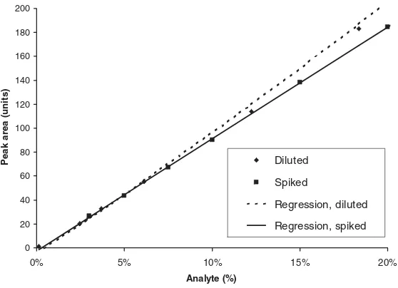
Measurements are inherently variable’ [16], i.e., the analytical data obtained scatter around the true value. The distribution of data can be visualised by histograms, i.e., plotting the frequency of the data within constant intervals (classes) throughout the whole data range observed. Such histograms can be generated using Microsoft Excel (Tools/Data Analysis/Histogram; the Analysis ToolPak can be installed by means of Tools/Add-Ins). Usually, the number of classes corresponds approximately to the square root of the number of data. Figure 2.1-1 shows clearly that a large number of data is required to obtain a clear picture. The data were obtained by recording the absorbance of a drug substance test solution at 291 nm for 60 minutes with a sampling rate of 10/s. Of course, over such a long time, an instrumental drift cannot be avoided. From 15 minutes onwards, the drift in the absorbance values was constant. Various time segments were further investigated and for the drift be-tween 35 and 60 minutes the lowest residual standard deviation of the regression line was observed. The data were corrected accordingly, i.e., the corrected data repre-sent the scattering of the absorbance values around the regression line of the drift. The mean and standard deviation of these 15 000 data were calculated to be 692 and 0.1774 mAU, respectively. The very small relative standard deviation of 0.026 % rep-resents only the detection variability of the spectrophotometer.

(34)

Probability density function:

fðxÞ ¼_r 1ffiffiffiffiffiffi

2p

p exp ðx lÞ2

2r2

Excel: f(x)=NORMDIST(x;l;r;FALSE) (2.1-1)

landrdenote the true (population) mean and standard deviation, and replacing in ExcelFALSE’ by TRUE’ will give the cumulative function.

An analytical measurement can be regarded as arandom samplingof data from the corresponding (normal) distribution of all possible data. This is illustrated in Figure 2.1-2, where randomly selected subsets of six subsequent data from the 15 000 absorbance values are presented.

But how do I know that my analysis results are normally distributed?

Although there are some statistical tools to test for normal distribution [16, or sta-tistical textbooks], they are not very suitable from a practical point of view where

0 2 4 6 8 10 12 14

691.5 691.9 692.3 692.7

n = 25

0 5 10 15 20 25 30

691.5 691.8 692.1 692.4

n = 100

0 20 40 60 80 100 120 140

691.5 691.8 692.0 692.2 692.5

n = 1000

0 50 100 150 200 250 300 350 400

691.5 691.8 692.0 692.2 692.5

n = 15 000

(35)

2 Performance Parameters, Calculations and Tests

there is only a small number of data. However, normal distribution can be assumed for the results of most physico-chemical analysis. Even if there is a minor deviation, regarding the large uncertainty of an experimental standard deviation (see Section 2.1.1.2), it will still provide a practical measure of the analytical variability. It is more important to verify the absence of systematic errors, for example, from degrading solutions, or insufficiently equilibrated systems, etc. This can be done in a very

straightforward way byvisual inspectionof the data for trends. If the scale is not too

large, the human eye is very sensitive in detecting trends and groupings in the experimental data. Therefore, experimental results should always be presented graphically.

Outliers

In the same way as non-random behaviour, a single datum which substantially devi-ates from the remaining data set, a so-called outlier, can influence both the mean

and the standard deviation strongly. There are several statisticaloutlier testsavailable,

but they suffer from the usual shortcomings of statistical significance tests (see Sec-tion 1.4.2). Most important, they cannot reveal the cause of the outlying result. The same practice as in pharmaceutical released testing, i.e., analytical results can only be invalidated if an analytical error can be assigned, should also be applied to valida-tion studies (see Chapter 10). However, these tests may be applied as a diagnostic

24

0 50 100 150 200 250 300 350 400

691.3 691.5 691.7 691.9 692.1 692.3 692.5 692.7

Absorbance (classes)

Frequency

Ratio SD/SDtrue

0.3

0.9

1.3

1.8

(36)

tool in an investigation (although often the visualeyeball’ test will reveal the same information). They may indicate that the data series is not representative. In such cases, the whole series should be repeated.

2.1.1.2 Standard Deviations

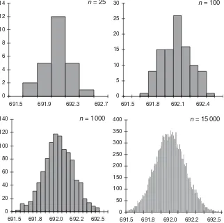
The standard deviation is an important parameter used to describe the width of the normal distribution, i.e., the degree of dispersion of the data. It corresponds to the horizontal distance between the apex and the inflection point of the Gaussian curve (Fig. 2.1-2, first pair of vertical dotted lines nearest to the mean solid line). The inter-val of–1 standard deviations around the true value includes just about two- thirds of all data belonging to this distribution. The two and three standard deviation inter-vals cover 95 % and 99.7 % of all data, respectively. The conclusion that almost all individual data of a population range within an interval of three standard deviations around both sides of the mean is the rationale for the so calledmethod capability index(see Section 1.4 and Chapter 10).

Variance and standard deviation: s2¼

P xi xx

ð Þ2

n 1

ð Þ s¼

ffiffiffiffi s2 p

(2.1-2)

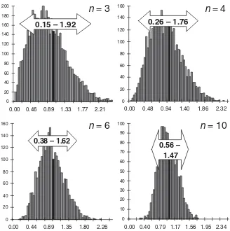
However, this relationship is based on the true standard deviation of the whole population (r). Small data sets, normally available in pharmaceutical analysis and validation, will vary within the theoretical possible range of the whole population, and their calculated (sample) standard deviation s (Eq. 2.1-2) will scatter rather widely. In Figure 2.1-2, five series of six subsequent values each, randomly selected from the 15 000 absorbance data, are shown. The calculated standard deviations vary from 30 % to 180 % of the true value. Note that these data sets are based on the same normal distribution! The variation of the standard deviation is only due to ran-dom variability in the data, i.e., it is statistically caused. The smaller the number of data, the higher is the variability of the calculated standard deviation (Fig. 2.1-3). For small numbers of data, the standard deviation distribution is skewed towards higher values, because the left side is limited to zero. Additionally, a larger proportion of the results is observed below the theoretical standard deviation (63 %, 60 %, 59 %, and 56 %, forn=3, 4, 6, and 10, respectively). Using more data to calculate the stan-dard deviation, the distribution becomes more narrow and symmetrical (Fig. 2.1-3,

n=6 and 10). Standard deviations calculated from six values (five degrees of freedom) were found up to 1.6 times the true value (estimated from the upper limit of the 95 %-range of all results, i.e., ignoring the upper 2.5 % of results). This is important to note when acceptance criteria for experimental standard deviations are to be defined, since here the upper limit of their distribution is relevant. These experi-mentally obtained ranges were confirmed by large data sets simulated from a nor-mal distribution (Table 2.1-1).

Variability limit (range): R¼z ffiffiffi

2 p

r_¼1:96 ffiffiffi

2 p

r»2:8r (2.1-3)

(37)

between two random values) that can be statistically expected. Equation (2.1-3) is based on the true standard deviation and the normal distribution. If individual

(experimental) standard deviations are used,zmust be replaced by the

correspond-ing Student-t-value. The analyst must be aware that the precision level determines the application of the variability limit, for example, with an injection repeatability, the maximum difference between two injections of the same solution is obtained, with a repeatability, the maximum range of independent sample preparations is obtained, etc.

If standard deviations are reported, it must be clearly stated to what they relate. Preferably, they should refer to single determinations. In this case, they provide information on the distribution of single data. If other calculations of the variability

26 0 20 40 60 80 200

0.00 0.46 0.89 1.33 1.77 2.21

n

= 3

0.15 – 1.92

0 20 40 60 80 100 120 140 160

0.00 0.48 0.94 1.40 1.86 2.32

n

= 4

0.26 – 1.76

0 20 40 60 80

0.00 0.44 0.89 1.35 1.80 2.26

n

= 6

0.38 – 1.62

0 10 20 30 40 50 60 70 80 90 100

0.00 0.40 0.79 1.17 1.56 1.95 2.34

n

= 10

0.56 –

1.47

180 160 140 120 100 160 140 120 100

(38)

Simulation of a normal distribution for a true meanland standard deviationr

(EXCEL):

x= NORMSINV(RAND())r+l (2.1-4)

are performed, such as repeated injections for each sample preparation, the preci-sion of the method (e.g. six times three sample preparations with duplicate injec-tions), the standard deviation of mean results, etc., then this should be clearly described; otherwise a meaningful interpretation is not possible. Unfortunately, this is a rather frequent shortcoming in the literature.

Usually, analytical variability is reported as a relative standard deviation (RSD), i.e., divided by the respective mean. This normalisation allows a direct comparison of precisions.

An analytical procedure is always composed of many individual steps. Each of them has its own variability, and their combination results in the overall variability. In this process, the variability can only increase, also known aserror propagation(for more details, see Section 6.2.2.1). The overall error can be calculated by the sum of all (relative) variances (uncertainty budget), also known as the bottom-up approach, to esti-matemeasurement uncertainty [21]. In pharmaceutical analysis, several contributing steps are usually grouped together in the experimental design, corresponding to the precision levels (see Section 2.1.2), this is also called the top-down approach.

2.1.1.3 Confidence Intervals

The (arithmetic) mean of the measurements is an estimate of the true value of a normal distribution. The latter can be expected in a certain interval around the sam-ple mean, the so-called confidence interval (Eq. 2.1-5). Because of the infinity of the normal distribution, data far away from the true value are theoretically possible (al-though with a very small probability, but this cannot predictwhensuch an event will

Table 2.1-1 Ranges of standard deviations calculated from simulated normally distributed data sets in relation to their sample size. The normally distributed data with a true standard deviation of 1 and a mean of 100 were calculated using Equation 2.1-4.

Sample size n (df = n-1)

Lower and upper limits between the indicated percentage of 50 000 calculated standard deviations were found

90 % 95 % 99 %

3 4 5 6 8 10 15 20

0.23 – 1.73 0.35 – 1.61 0.42 – 1.54 0.48 – 1.49 0.56 – 1.42 0.61 – 1.37 0.69 – 1.30 0.73 – 1.26

0.16 – 1.93 0.27 – 1.77 0.35 – 1.67 0.41 – 1.60 0.49 – 1.51 0.55 – 1.45 0.63 – 1.37 0.69 – 1.32

(39)

happen), the expectation needs to be restricted to a practical range. This is represented

by the error probabilitya, i.e., the part under the Gaussian curve, which is ignored, or

the statistical confidence (or significance) levelP(withP=100-a). Often, a 95 % level is

chosen. TheStudent-t-factoris a correction for the (un)reliability of the experimental

standard deviation obtained from a finite sample size (or strictly the underlying

distribu-tion). The term (s/n) is also called thestandard error of the meanand represents the

variability connected to the distribution of means. Compared to the distribution of sin-gle datum, the variability of the mean is reduced, as illustrated in Figure 2.1-2 (dia-monds vs. squares). The width of the confidence interval is dependent on the number of data (Fig. 2.1-4A). The more measurements that are performed, the better the mean estimates the true value. For an infinite number of data, the confidence interval of the mean approaches zero. As the confidence interval represents the range where the true value can be expected, this parameter may be useful in an out-of specification inves-tigation (if no analytical error can be assigned) to assess whether or not a batch fail-ure has occurred. If the whole confidence interval is within the acceptance limits of the specification, the true value can be expected to conform.

Confidence intervals:

of a mean CLðPÞ_x¼xx– s tðP;dfffiffiffi Þ

n

p (2.1-5)

of a standard deviation: CLðPÞ_s_;_lower¼ s

ffiffiffiffiffiffiffiffiffiffiffiffiffiffiffiffiffiffiffiffiffiffiffiffi df

v2_ð₁ _P_;_df_Þ

s

(2.1-6)

CLðPÞs;upper¼ s

ffiffiffiffiffiffiffiffiffiffiffiffiffiffiffiffiffiffi df

v2_ð_P_;_df_Þ