WEATHER MONITORING MODEL BASED ON SATELLITE DATA
(Model Pemantauan Cuaca Berdasar pada Data Satelit) Idung Risdiyanto1)
1)
Staff inGeophysics and Meteorology Department, Faculty of Math and Natural Science, Bogor Agriculture University
Weather monitoring model is closely related to the problem of objective analysis of the field of meteorology. The amount of meteorological data is quite substantial and hence the processing of these data is one of primary problems is dynamic meteorology. Therefore, a weather system model must consider atmospheric process, which can be built by mechanistic model rather than statistical approach. Integration of numerical model and spatial model will produce spatial weather information. It should be managed in one computerized system called as an information system for weather monitoring. The approach of the research was divided into five tasks. First task was satellite data capturing and extracting, second was development of numerical modeling based on dynamic and thermodynamic of atmospheric process, third was integration of numerical modeling and geographic information system in the spatial model, fourth was to develop graphical user interface and the fifth task was application of system in the real-world. Temporal resolution of this model is one day, however, in reality weather is temporal state of atmosphere condition that change any time. Moreover, this model only describes weather condition when data satellite on the day could be captured. Therefore, to increase the temporal resolution of this model, the input data could be added or integrated with other satellite data such as GMS satellite that has one-hour temporal resolution. Spatial resolution in this model is 50x50 kilometers square for global and 8x8 kilometers for regional area. Actually, for the spatial resolution, this model has been prepared as NOAA’s spatial resolution. This model cannot simulate vertical distribution of atmosphere, so, it does not give information about relative humidity and precipitation. If air movement in vertical area could be simulated, the dew point temperature and lighting condensation level would be known therefore the relative humidity and precipitation could be predicted.
Keywords : atmosphere , information system, resolution, satellite data, spatial model,
INTRODUCTION
Weather is a temporal state of surface atmosphere and is one of natural phenomena
that influences human activity and environmental conditions. Therefore, we could consider
weather as a natural system with elements or factors that represent weather condition. If we
called weather as a system, we could build a model as simplification of the weather system. A
model of weather system may be used for understanding weather phenomena, monitoring and
predicting the weather condition.
_____________
The progress of computer and geographical information technologies has supported the
development weather prediction model. Weather system considers temporal and spatial
dimension. There is which lead to representation of four dimensions. They comprise three
spatial dimensions and one temporal dimension. Weather system model can be developed by
integrating numerical model and geographic information system that can be used for weather
monitoring or prediction.
Weather monitoring model is closely related to the problem of objective analysis of the
field of meteorology. The amount of meteorological data is quite substantial and hence the
processing of these data is one of primary problems is dynamic meteorology. Therefore, a
weather system model must consider atmospheric process, which can be built by mechanistic
model rather than statistical approach. This model will be an integration of spatial model to find
information based on location and time of weather condition. In this research, model of weather
system will be constructed to monitor a daily weather conditions. Integration of numerical model
(as mechanistic model) and spatial model will produce spatial weather information. It should be
managed in one computerized system called as an information system for weather monitoring.
OBJECTIVES
The main objective of the study was to develop an information system for weather
monitoring based on numerical model and geography information system. In addition, this
objective could be described as specific objectives as follows:
To develop model design for simulating weather condition based on surface
temperature data that was extracted from NOAA AVHRR Local Area Coverage satellite
and digital elevation data (DEM)
To create algorithm and script of program for extracting NOAA AVHRR Local Area
Coverage satellite data.
To translate model design of weather monitoring system into computer algorithm
To build a package of application software for implementing model design for
MATERIAL AND METHODS Location and Duration
The research was conducted at Laboratory of Master of Science in Information
Technology for Natural Resources Management (MIT) and Agrisoft Laboratory at
SEAMEO-BIOTROP Bogor. The study area is 60°N-60°S latitude / 0°E-270°E longitude and
23.5°N-23.5°S latitude / 82°E-164°E longitude.
Research Area
The research area cover the development of weather monitoring model using
integration of three different approach, namely numerical modeling of weather variables, spatial
modeling for weather mapping and the development of graphical user interface that integrates
numerical and spatial models.
Required Tools
In this research, we use some supporting tools of software and hardware.
Software Utilities
MS Visual Basic 6.0 Developed numerical and spatial modeling, spatial database
ESRI MapObjects LT Developed spatial modeling
MS C++ Develop numerical and spatial modeling and satellite data
processing
MS Acces 2000 Database building
PC Arc/Info 3.51 Spatial data collecting, capturing and processing
ArcView 3.1 Spatial data collecting, capturing and processing
ER Mapper 5.5 Image data collecting, capturing and processing
MovingMap ActiveX Displayed result of model
Hardware
PC Pentium III 730 (over clock) MHz 128 MB RAM Computer Server Pentium III 450 MHz 64 MB RAM Printer Color
Data Sources
The research employed three main source of data, namely :
NOAA satellite raw data ( Local Area Coverage -LAC)
Digital elevation model (DEM) data (scale: 1:1000000)
Methodology
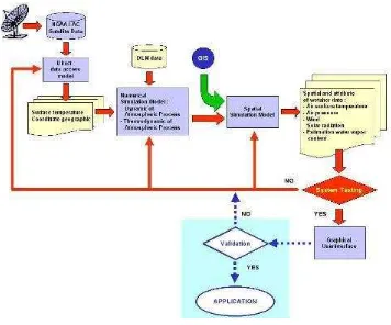
The approach of the research was divided into five tasks. First task was satellite data
capturing and extracting, second task was development of numerical modeling based on
dynamic and thermodynamic of atmospheric process, third task was integration of numerical
modeling and geographic information system in the spatial model, fourth task was to develop
graphical user interface and the fifth task was application of system in the real-world. The
method is presented in Figure 1. This research did not conduct model validation, due to
limitation of measured data such as those were by radio-sonde and time constraint.
Satellite data capturing and extracting
Satellite data in this research were derived from NOAA-14 satellite. Those data were
obtained from Internet in the form raw data which specific format data. Specific format data
refers to satellite data that were derived by different machine language in one metadata. NOAA
satellite data has three main formats; signed integer, unsigned integer and ASCII format. To
extract information from satellite, we build a model for direct accessing using computer program.
The program will translate information of raw data to numerical information in text format by
which the data can be read by the numerical model.
Numerical model for atmospheric process
The numerical model for atmospheric process consider thermodynamic and dynamic of
atmospheric processes. The basic task of this modeling is to formulate theoretical model of the
dynamic and thermodynamic of atmospheric process for the purpose of creating justifiable
weather system. This research attempts to formulate a theoretical model of weather system on
the basis of hydrodynamic equation in a way, which leads to the simultaneous fulfillment of the
conservation laws of the total momentum, the mass, and the total energy of a system.
Integration numerical modeling and geographic information system
Integration of numerical model and geographic information system is to produce spatial
information. Spatial information describe data of the local climate conditions of averages of
temperature based on altitude, normal conditions for energy balance based on latitude and
longitude of locations. These data will be integrated with the data that provide by the numerical
model. The integration of both data was handled by using MS Visual Basic computer program.
The result of the integration is weather monitoring consisting attribute of weather element which
Graphical user interface
In this research, the user interfaces was build with emphasis on the graphical user
interfaces and standard windowing environment to enable the users and operators access or
use the system easier. In this case, the user interface customizing by MS Visual Basic Program.
.
Figure 1. Block diagram of research methodology
RESULT AND DISCUSSION
This model was designed to simulate five weather elements. There are air surface
temperature, air pressure, wind, solar radiations and estimation of water vapor content. Each
weather element is simulated in separate module of the entire computer program.
Air Surface Temperature
The weather numerical model in this research used temperature data as the main input
for simulating other weather element data. Source of temperature data provide two types of raw
data. Those are NOAA satellite data and digital elevation model (DEM) data. NOAA satellite
format. The surface temperature from NOAA data and DEM data was interpolated. The
interpolation method is a kriging to estimation the temperature data for each parcel. The
interpolation method is a kriging, a geostatistical gridding method that has been proven useful
and popular in many fields.
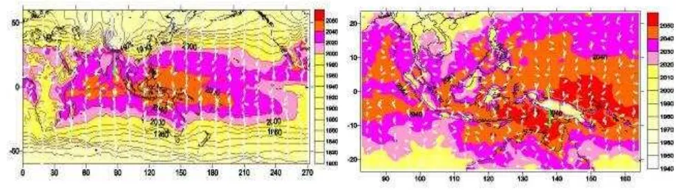
Figure 2. Logical flow to produce surface temperature data and Map of global surface temperature 02 June 2001 at global and regional area
This module produces two surface temperature data for each day. They are global and
regional air surface temperature. The global surface temperature data has 50 x 50 kilometers
square resolution while regional surface temperature has 8 x 8 kilometers square resolutions.
Global surface temperature provides distribution of surface temperature value in tropical area.
Atmospheric Pressure
The input data of the air pressure module are geographical coordinate and surface
temperature of air parcel. The assumptions in this model are :
acceleration of gravity (g0) : 9.80665 ms -2
air parcel condition is hydrostatic equilibrium
Initialization of air pressure (P0) :1013.25 mbar
Atmosphere height is less than 11 km which has the certain lapse rate and the value of
Vertical distribution of atmosphere pressure
Vertical distributions of atmosphere module predict the distance of a certain pressure
height from sea surface. Based on the above assumptions, module output is a geopotential
height that could be achieved by each a pressure layers in the atmosphere. In this module the
atmosphere divided into 9 layers of pressure. There are 900 mb, 850 mb, 800 mb, 750 mb, 700
mb, 650 mb, 600 mb, 550 mb and 500 mb. The module to calculate geopotential height is
derived from Poison’s equation shown in Eq. 1.
The map of geopotential height with vector that represents direction of air movement is
shown in Figure 3. Air moves from cold region into warm region. Cold air region is shown by
less geopotential height while warm air region is represented by higher geopotential height. As
a result, air mass from North and South sub tropical will move into tropical region (Figure 3).
The velocity of air movement depends on distance between isolines of geopotential height
called as horizontal gradient of geopotential height. The air movement velocity will increases
with less distance between of the isolines. The velocity and direction of air movement is
explained in different section 4.3.
p : certain atmosphere height (mbar) T0 : surface temperature
g : gravity (ms-2
)
Figure 3. Variations of geopotential height (m) and estimation air movement
Horizontal distribution of atmosphere pressure
In this model, horizontal distribution or variations of atmosphere pressure are defined as
differences pressure value between air parcels on the constant height from sea surface level.
The warm air has higher elevation than cold air. The high air column presents convergent area
with upward air movement, whereas low air column presents divergent area with downward air
movement. This model describes the direction of pressure gradient force at the horizontal plate.
The pressure value is calculated using an equation that is derived from Poison’s equation then
simulated using array of pressure until constant height to be achieved. The result of this module
is pressure value at constant height (z) for each air parcel. Commonly, the discussion of
meteorology infrequently uses this method to presents distribution of pressure. However, this
model is not supported by observation data on the surface. Therefore in this research we used
it.
The output of model (isobar chart) is the air pressure pattern on a constant height chart
(for example if height = 3 km). Whether this type of chart is not common in meteorology, but it
is frequently used when we have to measure the actual air pressure value at many station by
using radio sonde. Figure 4a presents an isobar chart on a constant height level (3000 meter)
of Indonesia’s Islands and it’s surrounding on December 02, 2000. The graph of the output
model presents that not all region which near 0° latitude has lower pressure then higher latitude
(see Figure 4b). It is a selected data from 105°E to 120°E longitude. If we compare with the
map data (Figure 4a) we will see that the land surface near 0° latitude is higher probability than
Figure 4. (a) Isobar (mb) chart (Z = 3000 m) on 2 December 2000 and (b) Variation
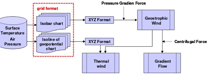
module simulated three types of wind; geostrophic wind, gradient flow and thermal wind, where
for each type of wind has the relation with the other types such as given by Figure 5.
Surface
Figure 5. Logical flow of wind module
All input data of wind model is independent data. It means, each of data depend on the
air parcel and does not has relation with other parcels, except, if those was interpolated.
Therefore, before calculated the direction and magnitude of wind, the model need a grid
relations to explain spatial and numerical derivative. When a numerical derivative is required, a
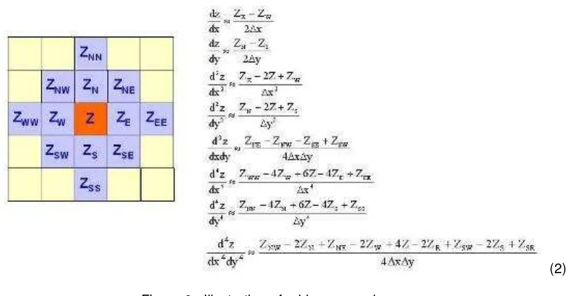
central difference formula is used in the grid computations process and uses "compass-based"
grid notation to indicate the neighboring grid nodes as presented in Figure 6. Using this grid
notation, we can derive the difference equation approximations for the necessary derivatives at
(2)
Figure 6. Illustration of grid compass-base
Geostrophic Wind
Based on balancing of pressure gradient force and Coriolis force, the magnitude of
geostrophic wind could be simulated with isobar chart as data input (in XYZ format data).
Magnitude of geostrophic wind is simulated using follows equations (derived from Eq. 2):
Vg : Magnitude of geostrophic wind (ms -1
)
: Air mass specific was calculated using the empirics equation as a function that provide by temperature and pressure at certain level (kg m-3
)
: Rotation rate of the earth ( 7.29 x 10⁻⁵
s-1
)
: Latitude position of the grid
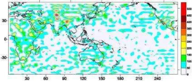
Simulation of geostropic wind is applied in global study area only. As we known that
geostropic wind has value more than zero if the latitude more than zero, otherwise it has
significant value in middle and high latitude area and its value limit to zero in low latitude area.
Figure 7 in below give an example of result simulation of geostropic wind velocity on June 02,
2001.
From Figure 8, almost area has velocity are less than 50 ms-1, especially in low latitudes.
Otherwise, in middle and high latitude, the geostropic wind velocity increase more than 500 ms-1
and it’s developed a form such as curve. This curve is a flow around high pressure or low
-pressure center. In this research could not identification that geostropic flow around high or low
pressure, so that, could not determine cyclone or anticyclone area and direction of geostropic
Figure 7. Velocity (ms-1) distribution of geostropic wind on June 02, 2001
simulation, it also uses central difference of grid notation using the first derivative of isobar. This
derivation refers to the basic equation as follows.
three-way balances of forces in cyclonic flow, i.e. centrifugal force, coriolis force, and pressure
gradient force. Therefore this simulation gives more detail in expressing an air movement (see
Figure 8).
Figure 8. Velocity (ms-1) distribution of gradient wind on June 02, 2001
In Figure 8, the wind gradient presents the distribution of wind velocity in low latitudes.
The highest velocity occurs mostly on land surface because the distance of isobar line is shorter
state presents the difference heat capacity that influences the surface temperature where finally
shows the different of air pressure on both surfaces.
Thermal Wind
The combination of hypsometric and geostrophic equations gives a thermal wind
equation which relates vertical shear of the geostrophic wind to horizontal temperature gradient.
This model uses central difference of grid notation from the first derivative of temperature
height. Therefore, the equation of thermal wind is given as follows.
y
The Wind Direction module considers about the differences between cold and warm air
or high and low pressure. Therefore, the input data for generating wind direction is geopotential
height (presents the differences of warm and cold air) and the isobar chart (presents the
differences of high and low pressure). Similar with the velocity of wind generation, wind
direction also uses “compass base” as a basic to derive a direction. The differences of pressure
for each parcel at certain elevation level from surface could be assumed as a terrain. Therefore,
the wind direction refers to the aspect of terrain.
The terrain aspect operation is calculated from the downhill direction of the steepest
slope at each grid node. This direction is perpendicular to the isobar lines at certain elevation on
the surface, and exactly opposite from the gradient direction. Terrain aspect values are reported
in azimuth, where 0 degrees points due North, and 90 degrees points due to East. The
operation is given by:
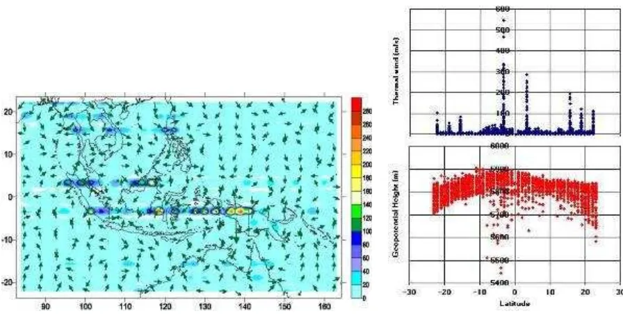
The velocity of thermal wind is given by Equation 5 while the direction is given by vector
calculation of differences geopotential height which is derived from hypsometric equation
(equation 6). In this research, the value of velocity was presented by color scale while arrow for
the direction of wind.
The simulations of thermal wind in regional area give more detail in result than
simulations in global area. In Figure 9a we see that the velocity of thermal wind is less than 20
has high geopotential height and high thermal gradient. Figure 9b presents the relation between
geopotential height and thermal wind velocity.
Figure 9. (a) The velocity and direction of thermal wind for South East Asia on June 02, 2001, (b) Relational geopotential height and thermal wind velocity
Solar Radiation
Solar radiations module was built as a function of coordinate geography, time and
surface temperature. Coordinate geography and time determines the potential value of solar
radiation which is receive by earth surface. Temperature of surface data is used to generate the
actual value when the satellite data was captured. Those all data will be combined with certain
physical equation of electromagnetic wave.
In this research, Plank’s equation is the first theory that is used to simulate the solar
radiance value. This equation describes the quantum theory about energy that is transmitted by
electromagnetic radiation in discrete unit (called photons). The second theory is blackbody
radiation. It is a hypothetical body comprising a sufficient number of molecules absorbing and
emitting electromagnetic radiation in all parts of the electromagnetic spectrum. In this model,
the known data is surface temperature data for each coordinate. By those two equations, we
can calculate the value of solar radiation on the earth surface. The surface temperature data,
which was produced from extracting satellite data, is a result of the infrared spectrum on certain
the equation to generate the solar energy value on the earth’s surface could be expressed as
follows.
2897 T hc
Q (7)
The simulations of solar energy on the earth surface is a calculation of surface
irradiance, therefore the result expresses an energy from reflectance of solar radiance and long
wave radiance of surface that is received by satellite sensor. It gives irradiance value and
maximum wavelength as an output of model.
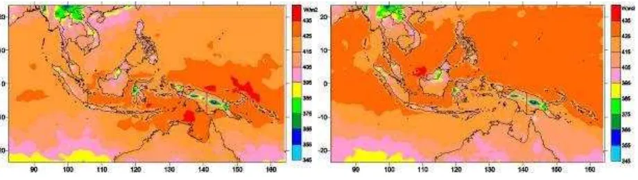
Regional study area gives more detail information. In this research, the solar energy
simulation is conducted on December 02, 2000 and June 02, 2001 where the results are
presented in Figure 10. From Figure 10, on December 02, 2000, the area South of equator
receives solar radiance more than the North area. In contrast, on June 02, 2001, the solar
radiance in North area is more than the South area. In addition, the area that has a high value
of solar irradiance on June is larger than on December.
Figure 10. Distribution of average solar energy (Wm-2) which has been receives by earth surface in regional area on (left) December 02, 2000 and (right) June 02, 2001.
Estimation of Water Vapor Content
Module of estimation of water vapor content consider about water vapor mass and
cloud distribution. Those variables can be predicted from vertical distribution of solar energy.
Cloud, water vapor and aerosol that are exist in the atmosphere influence the radiation transfer
process, because they absorb and reflect some part of solar radiation.
The model of water vapor content estimation was build based on the mechanism of
energy transfer as the basis to estimate the water vapor content. The assumption was used in
component that has to be taken into account as atmosphere content. Another assumption is
constant in volume, therefore, the specific heat of water vapor used the value is 1463 J kg-1 K-1.
The solar energy was absorbing by atmosphere could be calculated such as below:
s a atm Q Q
Q (8)
The solar energy, which receives by earth surface, was substituted by using equation 7.
2897 T hc Q
Q s
a
atm (9)
Qa is potential energy that receives on top atmosphere and as a function of latitude, solar
declination angle and day. The equation is given by:
H
sin
sin
cos
cos
sin
H
6258
.
0
Q
a
(10)Based on equation 4.17 can be seen that if absorption solar energy by atmosphere is high, it is
presenting the high water vapor mass. The value of water vapor mass on certain area can be
used as indicator to predict precipitations, because the high value will be increasing growing
cloud. So, to get estimation of water vapor content in the atmosphere can used ratio between
energy that absorb by atmosphere and energy that receive on top atmosphere is given by:
%
100
x
Q
Q
WV
a atm
p
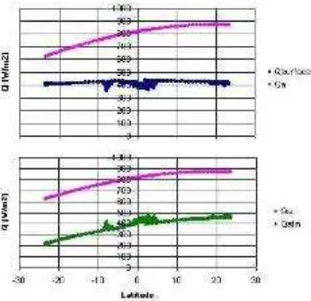
(11)The result of water vapor content estimation can be seen in Figure 11. Its express two
map, first map is condition on December 02, 2000 and second map is condition on June 02,
2001. Although just express solar radiance that absorb by the atmosphere, it could be used as
assumption water vapor content in the atmosphere. Figure 12 is shown the solar radiance that
absorbing by atmosphere. Qa is solar radiance before it was absorb by atmosphere and Qatm
is solar radiance that was absorbing by atmosphere.
Actually, in this research was not done simulations to get water vapor mass. If it wants
to calculate water content mass, so, it should consider about vertical distribution of air density
Figure 11. Estimation of relative water vapor content in the atmosphere (left December 02, 2000, right – 02 June 2001)
Figure 12. Sample of solar radiance on surface, atmosphere and on top atmosphere (Wm-2)
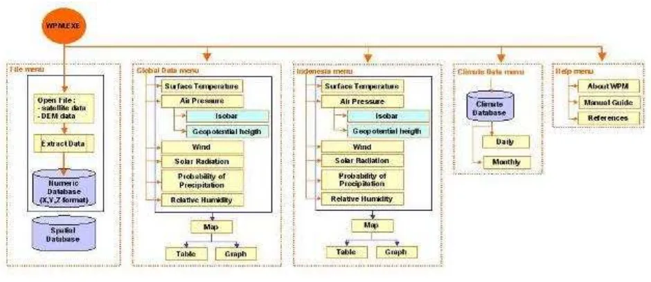
Graphical User Interface
In this research, a mode of user interface for weather prediction model is a graphical user
interface (GUI) and it was build as a packet software application. It was written in Visual Basic
6.0 and was supporting some library file and activeX from other software. In this GUI, there are
four major tasks that have to be handled. The first task is file management, second task is
global data presenting, third task is Indonesia data presenting and the last one is description
about this software and model. Each of tasks was presenting as menu of the application
Figure 13. Graphical user interface menu
To present the result of model, GUI was build with three displaying as layout; there are
map, table and graph or chart. The map was build with add the Surfer Library into project
reference and Moving Map activeX into project component of Visual Basic. Surfer library was
used for create griding file and produce map of weather element which was overlaying with
base map. Moving map activeX was used to displaying the map which was created by surfer
library and has the property such as zooming out, zooming in and showing coordinate value of
the map. Table and chart of weather element was building by using available activeX in Visual
Basic, their area MS Flexgrid and MS Chart.
CONCLUSIONS AND RECOMMENDATIONS
This research uses three techniques (modeling, geographic information system and
remote sensing) to develop weather monitoring application software as implementation of
information technology. Modeling that was used in this research is mechanistic model which
describe atmospheric process and give weather element value as an output. Geographic
information system was used to create spatial model to give geo-reference for the result of
mechanistic model, therefore it is enable to be plotted on the map. Remote sensing technology
was used to capture NOAA satellite data and extract it to produce a radians value as an input of
mechanistic model.
The weather monitoring application software consists of three model. The first
automatically. The second model is numerical weather system model which is used to simulated
weather element data. The last model is spatial model which is used to build relationship of
weather element data between pixel or area of air column. By this software, users could get the
information of weather elements data such as air surface temperature, air pressure, wind, solar
radiation and water vapor content estimation.
As a model, it has some weakness such as temporal resolution, spatial resolution and
vertical distribution process of atmosphere. Temporal resolution of this model is one day,
however, in reality, weather is temporal state of atmosphere condition that change any time.
Moreover, this model only describes weather condition when data satellite on the day could be
captured. Therefore, to increase the temporal resolution of this model, the input data could be
added or integrated with other satellite data such as GMS satellite that has one-hour temporal
resolution.
Spatial resolution that was used in this model is 50x50 kilometers square for global area
and 8x8 kilometers for regional area. Actually, for the spatial resolution, this model has been
prepared as NOAA’s spatial resolution. However, in this research, the computer processor and
memory is not adequate to run the software in NOAA’s spatial resolution. Therefore, it is highly
recommended to use more powerful computer system.
This model cannot simulate vertical distribution of atmosphere, so, it does not give
information about relative humidity and precipitation. If air movement in vertical area could be
simulated, the dew point temperature and lighting condensation level would be known therefore
the relative humidity and precipitation could be predicted.
Considering with weather prediction, this model could be used as initialization to predict
the next weather condition (12 hour, 24 hour or 48 hour). However, this model must be
validated using radio-sonde and surface data (weather station data). Therefore, this research
should be continued with add new method to simulate vertical distribution of atmosphere and
REFERENCES
Andersson, K. 1999. DRAFT-NOAA AVHRR Data Processing Software User’s Guide (Ver 2.22). VTT Automation. http://www.vtt.fi/aut/rs/docs/avhrr_guide.html
Aronoff. A., Geographic Information System: A Management Perspective. WDL Publications Ottawa, Canada.
Burrough, P.A., 1985. Principles of Geographical Information Systems for Land Resources Assesment. Clarendon Press. Oxord.
Demers. M.N., 1997. Fundamentals Of Geographic Information System. New Mexico State University. John Wiley & Son, INC.
De By, R.A, 2000. Principles of Geographic System; An Introductory Textbook. The International Instiute For Aerospace Survey and Earth Science (ITC), Nederlands.
Finizio, N and G. Ladas. 1988. Ordinary Differential Equation with Modern Application, 2nd edition. Erlangga. Bandung. Indonesia.
Holton, J.R. 1992. An introduction to Dynamic Meteorology, 3th edition. Academic Press, Inc. New York. USA.
Hu, Y and B.A. Wielicky. 1996. Radiance computation for randomly distributed clouds with discrete ordinate method, part 1: Theory and Model. Computer Based Learning Unit. University of Leeds. United Kingdom.
Manurung, P. 2000. Studi Kandungan Uap Air Regional Indonesia dengan GPS (Study of Regional Precipitable Water Vapour in Indonesia with GPS). Riset Unggulan Terpadu VI-Teknologi Perlindungan Lingkungan. Dewan Riset Nasional. Jakarta. Indonesia.
Marchuk, G.I. 1974. Numerical Methods in Weather Prediction. Academic Press. London.
Menzel, P and K. Strabala. 1997. Cloud top properties and cloud phase algorithm theoretical basis document. Institute for Meteorological Satellite Studies. University of Wisconsin. Madison. USA.
NOAA. 1999. NOAA users guide. NOAA Satellite Active Archive. http://www.saa.noaa.gov
O’Dempsey, T. 2000. Managing Accuracy of Spatial Data, White Paper. ESRI South Asia Pte
Ltd.
Pasquill, F. 1977. Atmospheric Diffusion; The Dispersion of Winborne Material from Industrial and Other Resource, 2th edition. Ellis Horwood Limited. John Wiley & Son. New York. USA .
Pawitan, H. 1989. Termodinamika Atmosfer (Atmospheric Thermodynamics). Institut Pertanian Bogor, Pusat Antar Universitas Ilmu Hayat. Direktorat Jenderal Pendidikan Tinggi. Departemen Pendidikan dan Kebudayaan. Bogor. Indonesia.
Raymond, D., S.Esbensen., M.Gregg and N. Shay. 2001. EPIC2001: Overview and Implementation plan.
Rogers, R.R. 1983. A short course in Cloud Physics. Pergamon Press. Oxford
Rosenberg, J.R., B.L. Blad and S.B. Verma. 1983. Microclimate; The Biological Environment, 2nd edition. A Wiley-Interscience Publication. New York.
Swartz, M.E. and Young, P.M. 1999. Instrument Qualification and Method Validation for Dissolution Assays With HPLC Analyses. Waters Corporation Milford.
http://www.waters.com/waters_website/applications/validate/Vldt_top.htm
.Tritton, D.J. 1977. Physical Fluid Dynamics. Van Nostrand Reinhold (UK) Co.Ltd. Wokingham-Berkshire. England.