THE PHYSICAL SCIENCES
Third Edition
MATHEMATICAL METHODS IN
THE PHYSICAL SCIENCES
Third Edition
PRODUCTION EDITOR Sarah Wolfman-Robichaud
MARKETING MANAGER Amanda Wygal
SENIOR DESIGNER Dawn Stanley
EDITORIAL ASSISTANT Krista Jarmas/Alyson Rentrop PRODUCTION MANAGER Jan Fisher/Publication Services
This book was set in 10/12 Computer Modern by Publication Services and printed and bound by R.R. Donnelley-Willard. The cover was printed by Lehigh Press.
This book is printed on acid free paper.
Copyright2006 John Wiley & Sons, Inc. All rights reserved. No part of this publication may be reproduced, stored in a retrieval system or transmitted in any form or by any means, electronic, mechanical, photocopying, recording, scanning, or otherwise, except as permitted under Sections 107 or 108 of the 1976 United States Copyright Act, without either the prior written permission of the Publisher, or authorization through payment of the appropriate per-copy fee to the Copyright Clearance Center, Inc., 222 Rosewood Drive, Danvers, MA 01923, (978)750-8400, fax (978)750-4470 or on the web at www.copyright.com. Requests to the Publisher for permission should be addressed to the Permissions Department, John Wiley & Sons, Inc., 111 River Street, Hoboken, NJ 07030-5774, (201)748-6011, fax (201)748-6008, or online at http://www.wiley.com/go/permissions.
To order books or for customer service please, call 1-800-CALL WILEY (225-5945). ISBN 0-471-19826-9
PREFACE
This book is particularly intended for the student with a year (or a year and a half) of calculus who wants to develop, in a short time, a basic competence in each of the many areas of mathematics needed in junior to senior-graduate courses in physics, chemistry, and engineering. Thus it is intended to be accessible to sophomores (or freshmen with AP calculus from high school). It may also be used effectively by a more advanced student to review half-forgotten topics or learn new ones, either by independent study or in a class. Although the book was written especially for students of the physical sciences, students in any field (say mathematics or mathematics for teaching) may find it useful to survey many topics or to obtain some knowledge of areas they do not have time to study in depth. Since theorems are stated carefully, such students should not need to unlearn anything in their later work.
The question of proper mathematical training for students in the physical sci-ences is of concern to both mathematicians and those who use mathematics in appli-cations. Some instructors may feel that if students are going to study mathematics at all, they should study it in careful and thorough detail. For the undergradu-ate physics, chemistry, or engineering student, this means either (1) learning more mathematics than a mathematics major or (2) learning a few areas of mathematics thoroughly and the others only from snatches in science courses. The second alter-native is often advocated; let me say why I think it is unsatisfactory. It is certainly true that motivation is increased by the immediate application of a mathematical technique, but there are a number of disadvantages:
1. The discussion of the mathematics is apt to be sketchy since that is not the primary concern.
2. Students are faced simultaneously with learning a new mathematical method and applying it to an area of science that is also new to them. Frequently the
difficulty in comprehending the new scientific area lies more in the distraction caused by poorly understood mathematics than it does in the new scientific ideas. 3. Students may meet what is actually the same mathematical principle in two different science courses without recognizing the connection, or even learn ap-parently contradictory theorems in the two courses! For example, in thermody-namics students learn that the integral of an exact differential around a closed path is always zero. In electricity or hydrodynamics, they run into2π
0 dθ, which is certainly the integral of an exact differential around a closed path but is not equal to zero!
Now it would be fine if every science student could take the separate mathematics courses in differential equations (ordinary and partial), advanced calculus, linear algebra, vector and tensor analysis, complex variables, Fourier series, probability, calculus of variations, special functions, and so on. However, most science students have neither the time nor the inclination to study that much mathematics, yet they are constantly hampered in their science courses for lack of the basic techniques of these subjects. It is the intent of this book to give these students enough background in each of the needed areas so that they can cope successfully with junior, senior, and beginning graduate courses in the physical sciences. I hope, also, that some students will be sufficiently intrigued by one or more of the fields of mathematics to pursue it futher.
It is clear that something must be omitted if so many topics are to be compressed into one course. I believe that two things can be left out without serious harm at this stage of a student’s work: generality, and detailed proofs. Stating and proving a theorem in its most general form is important to the mathematician and to the advanced student, but it is often unnecessary and may be confusing to the more elementary student. This is not in the least to say that science students have no use for careful mathematics. Scientists, even more than pure mathematicians, need careful statements of the limits of applicability of mathematical processes so that they can use them with confidence without having to supply proof of their validity. Consequently I have endeavored to give accurate statements of the needed theorems, although often for special cases or without proof. Interested students can easily find more detail in textbooks in the special fields.
Mathematical physics texts at the senior-graduate level are able to assume a degree of mathematical sophistication and knowledge of advanced physics not yet attained by students at the sophomore level. Yet such students, if given simple and clear explanations, can readily master the techniques we cover in this text. (They not only can, but will have to in one way or another, if they are going to pass their junior and senior physics courses!) These students are not ready for detailed applications—these they will get in their science courses—but they do need and want to be given some idea of the use of the methods they are studying, and some simple applications. This I have tried to do for each new topic.
For those of you familiar with the second edition, let me outline the changes for the third:
Preface ix
Chapter 12 (Series solutions) and Chapter 13 (Partial differential equations). 2. Again, prompted by several requests, I have moved Fourier integrals back to the
Fourier series Chapter 7. Since this breaks up the integral transforms chapter (old Chapter 15), I decided to abandon that chapter and move the Laplace transform and Dirac delta function material back to the ordinary differential equations Chapter 8. I have also amplified the treatment of the delta function. 3. The Probability chapter (old Chapter 16) now becomes Chapter 15. Here I have
changed the title to Probability and Statistics, and have revised the latter part of the chapter to emphasize its purpose, namely to clarify for students the theory behind the rules they learn for handling experimental data.
4. The very rapid development of technological aids to computation poses a steady question for instructors as to their best use. Without selecting any particular Computer Algebra System, I have simply tried for each topic to point out to students both the usefulness and the pitfalls of computer use. (Please see my comments at the end of ”To the Student” just ahead.)
The material in the text is so arranged that students who study the chapters in order will have the necessary background at each stage. However, it is not always either necessary or desirable to follow the text order. Let me suggest some rearrangements I have found useful. If students have previously studied the material in any of chapters 1, 3, 4, 5, 6, or 8 (in such courses as second-year calculus, differential equations, linear algebra), then the corresponding chapter(s) could be omitted, used for reference, or, preferably, be reviewed briefly with emphasis on problem solving. Students may know Taylor’s theorem, for example, but have little skill in using series approximations; they may know the theory of multiple integrals, but find it difficult to set up a double integral for the moment of inertia of a spherical shell; they may know existence theorems for differential equations, but have little skill in solving, say, y′′+y = xsinx. Problem solving is the essential core of a course on Mathematical Methods.
After Chapters 7 (Fourier Series) and 8 (Ordinary Differential Equations) I like to cover the first four sections of Chapter 13 (Partial Differential Equations). This gives students an introduction to Partial Differential Equations but requires only the use of Fourier series expansions. Later on, after studying Chapter 12, students can return to complete Chapter 13. Chapter 15 (Probability and Statistics) is almost independent of the rest of the text; I have covered this material anywhere from the beginning to the end of a one-year course.
It has been gratifying to hear the enthusiastic responses to the first two editions, and I hope that this third edition will prove even more useful. I want to thank many readers for helpful suggestions and I will appreciate any further comments. If you find misprints, please send them to me at [email protected]. I also want to thank the University of Washington physics students who were my LATEX typists: Toshiko Asai, Jeff Sherman, and Jeffrey Frasca. And I especially want to thank my son, Harold P. Boas, both for mathematical consultations, and for his expert help with LATEX problems.
Instructors who have adopted the book for a class should consult the publisher about an Instructor’s Answer Book, and about a list correlating 2nd and 3rd edition problem numbers for problems which appear in both editions.
TO THE STUDENT
As you start each topic in this book, you will no doubt wonder and ask “Just why should I study this subject and what use does it have in applications?” There is a story about a young mathematics instructor who asked an older professor “What do you say when students ask about the practical applications of some mathematical topic?” The experienced professor said “I tell them!” This text tries to follow that advice. However, you must on your part be reasonable in your request. It is not possible in one book or course to cover both the mathematical methods and very many detailed applications of them. You will have to be content with some information as to the areas of application of each topic and some of the simpler applications. In your later courses, you will then use these techniques in more advanced applications. At that point you can concentrate on the physical application instead of being distracted by learning new mathematical methods.
One point about your study of this material cannot be emphasized too strongly: To use mathematics effectively in applications, you need not just knowledge butskill. Skill can be obtained only through practice. You can obtain a certain superficial knowledge of mathematics by listening to lectures, but you cannot obtainskill this way. How many students have I heard say “It looks so easy when you do it,” or “I understand it but I can’t do the problems!” Such statements show lack of practice and consequent lack of skill. Theonly way to develop the skill necessary to use this material in your later courses is to practice by solving many problems. Always study with pencil and paper at hand. Don’t just read through a solved problem—try to do it yourself! Then solve some similar ones from the problem set for that section,
trying to choose the most appropriate method from the solved examples. See the Answers to Selected Problems and check your answers to any problems listed there. If you meet an unfamiliar term, look for it in the Index (or in a dictionary if it is nontechnical).
My students tell me that one of my most frequent comments to them is “You’re working too hard.” There is no merit in spending hours producing a solution to a problem that can be done by a better method in a few minutes. Please ignore anyone who disparages problem-solving techniques as “tricks” or “shortcuts.” You will find that the more able you are to choose effective methods of solving problems in your science courses, the easier it will be for you to master new material. But this means practice, practice, practice! The only way to learn to solve problems is to solve problems. In this text, you will find both drill problems and harder, more challenging problems. You should not feel satisfied with your study of a chapter until you can solve a reasonable number of these problems.
You may be thinking “I don’t really need to study this—my computer will solve all these problems for me.” Now Computer Algebra Systems are wonderful—as you know, they save you a lot of laborious calculation and quickly plot graphs which clarify a problem. But a computer is a tool; you are the one in charge. A very perceptive student recently said to me (about the use of a computer for a special project): “First you learn how to do it; then you see what the computer can do to make it easier.” Quite so! A very effective way to study a new technique is to do some simple problems by hand in order to understand the process, and compare your results with a computer solution. You will then be better able to use the method to set up and solve similar more complicated applied problems in your advanced courses. So, in one problem set after another, I will remind you that the point of solving some simple problems is not to get an answer (which a computer will easily supply) but rather to learn the ideas and techniques which will be so useful in your later courses.
CONTENTS
1 INFINITE SERIES, POWER SERIES 1
1. The Geometric Series 1 2. Definitions and Notation 4 3. Applications of Series 6
4. Convergent and Divergent Series 6
5. Testing Series for Convergence; the Preliminary Test 9
6. Convergence Tests for Series of Positive Terms: Absolute Convergence 10 A. The Comparison Test 10
B. The Integral Test 11 C. The Ratio Test 13
D. A Special Comparison Test 15 7. Alternating Series 17
8. Conditionally Convergent Series 18 9. Useful Facts About Series 19
10. Power Series; Interval of Convergence 20 11. Theorems About Power Series 23 12. Expanding Functions in Power Series 23
13. Techniques for Obtaining Power Series Expansions 25
A. Multiplying a Series by a Polynomial or by Another Series 26 B. Division of Two Series or of a Series by a Polynomial 27
C. Binomial Series 28
D. Substitution of a Polynomial or a Series for the Variable in Another Series 29
E. Combination of Methods 30
F. Taylor Series Using the Basic Maclaurin Series 30 G. Using a Computer 31
14. Accuracy of Series Approximations 33 15. Some Uses of Series 36
16. Miscellaneous Problems 44
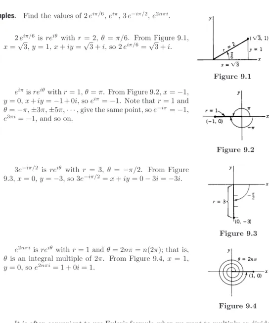
2 COMPLEX NUMBERS 46
1. Introduction 46
2. Real and Imaginary Parts of a Complex Number 47 3. The Complex Plane 47
4. Terminology and Notation 49 5. Complex Algebra 51
A. Simplifying tox+iy form 51
B. Complex Conjugate of a Complex Expression 52 C. Finding the Absolute Value of z 53
D. Complex Equations 54 E. Graphs 54
F. Physical Applications 55 6. Complex Infinite Series 56
7. Complex Power Series; Disk of Convergence 58 8. Elementary Functions of Complex Numbers 60 9. Euler’s Formula 61
10. Powers and Roots of Complex Numbers 64 11. The Exponential and Trigonometric Functions 67 12. Hyperbolic Functions 70
13. Logarithms 72
14. Complex Roots and Powers 73
15. Inverse Trigonometric and Hyperbolic Functions 74 16. Some Applications 76
17. Miscellaneous Problems 80
3 LINEAR ALGEBRA 82
1. Introduction 82
2. Matrices; Row Reduction 83 3. Determinants; Cramer’s Rule 89 4. Vectors 96
5. Lines and Planes 106 6. Matrix Operations 114
7. Linear Combinations, Linear Functions, Linear Operators 124 8. Linear Dependence and Independence 132
9. Special Matrices and Formulas 137 10. Linear Vector Spaces 142
Contents xv
13. A Brief Introduction to Groups 172 14. General Vector Spaces 179
15. Miscellaneous Problems 184
4 PARTIAL DIFFERENTIATION 188
1. Introduction and Notation 188 2. Power Series in Two Variables 191 3. Total Differentials 193
4. Approximations using Differentials 196
5. Chain Rule or Differentiating a Function of a Function 199 6. Implicit Differentiation 202
7. More Chain Rule 203
8. Application of Partial Differentiation to Maximum and Minimum Problems 211
9. Maximum and Minimum Problems with Constraints; Lagrange Multipliers 214 10. Endpoint or Boundary Point Problems 223
11. Change of Variables 228
12. Differentiation of Integrals; Leibniz’ Rule 233 13. Miscellaneous problems 238
5 MULTIPLE INTEGRALS 241
1. Introduction 241
2. Double and Triple Integrals 242
3. Applications of Integration; Single and Multiple Integrals 249 4. Change of Variables in Integrals; Jacobians 258
5. Surface Integrals 270 6. Miscellaneous Problems 273
6 VECTOR ANALYSIS 276
1. Introduction 276
2. Applications of Vector Multiplication 276 3. Triple Products 278
4. Differentiation of Vectors 285 5. Fields 289
6. Directional Derivative; Gradient 290 7. Some Other Expressions Involving∇ 296 8. Line Integrals 299
9. Green’s Theorem in the Plane 309
10. The Divergence and the Divergence Theorem 314 11. The Curl and Stokes’ Theorem 324
12. Miscellaneous Problems 336
7 FOURIER SERIES AND TRANSFORMS 340
1. Introduction 340
2. Simple Harmonic Motion and Wave Motion; Periodic Functions 340 3. Applications of Fourier Series 345
5. Fourier Coefficients 350 6. Dirichlet Conditions 355
7. Complex Form of Fourier Series 358 8. Other Intervals 360
9. Even and Odd Functions 364 10. An Application to Sound 372 11. Parseval’s Theorem 375 12. Fourier Transforms 378 13. Miscellaneous Problems 386
8 ORDINARY DIFFERENTIAL EQUATIONS 390
1. Introduction 390 2. Separable Equations 395
3. Linear First-Order Equations 401
4. Other Methods for First-Order Equations 404
5. Second-Order Linear Equations with Constant Coefficients and Zero Right-Hand
Side 408
6. Second-Order Linear Equations with Constant Coefficients and Right-Hand Side Not Zero 417
7. Other Second-Order Equations 430 8. The Laplace Transform 437
9. Solution of Differential Equations by Laplace Transforms 440 10. Convolution 444
11. The Dirac Delta Function 449
12. A Brief Introduction to Green Functions 461 13. Miscellaneous Problems 466
9 CALCULUS OF VARIATIONS 472
1. Introduction 472 2. The Euler Equation 474 3. Using the Euler Equation 478
4. The Brachistochrone Problem; Cycloids 482
5. Several Dependent Variables; Lagrange’s Equations 485 6. Isoperimetric Problems 491
7. Variational Notation 493 8. Miscellaneous Problems 494
10 TENSOR ANALYSIS 496
1. Introduction 496 2. Cartesian Tensors 498
3. Tensor Notation and Operations 502 4. Inertia Tensor 505
5. Kronecker Delta and Levi-Civita Symbol 508 6. Pseudovectors and Pseudotensors 514 7. More About Applications 518 8. Curvilinear Coordinates 521
Contents xvii
10. Non-Cartesian Tensors 529 11. Miscellaneous Problems 535
11 SPECIAL FUNCTIONS 537
1. Introduction 537
2. The Factorial Function 538
3. Definition of the Gamma Function; Recursion Relation 538 4. The Gamma Function of Negative Numbers 540
5. Some Important Formulas Involving Gamma Functions 541 6. Beta Functions 542
7. Beta Functions in Terms of Gamma Functions 543 8. The Simple Pendulum 545
9. The Error Function 547 10. Asymptotic Series 549 11. Stirling’s Formula 552
12. Elliptic Integrals and Functions 554 13. Miscellaneous Problems 560
12 SERIES SOLUTIONS OF DIFFERENTIAL EQUATIONS;
LEGENDRE, BESSEL, HERMITE, AND LAGUERRE
FUNCTIONS 562
1. Introduction 562 2. Legendre’s Equation 564
3. Leibniz’ Rule for Differentiating Products 567 4. Rodrigues’ Formula 568
5. Generating Function for Legendre Polynomials 569 6. Complete Sets of Orthogonal Functions 575 7. Orthogonality of the Legendre Polynomials 577 8. Normalization of the Legendre Polynomials 578 9. Legendre Series 580
10. The Associated Legendre Functions 583
11. Generalized Power Series or the Method of Frobenius 585 12. Bessel’s Equation 587
13. The Second Solution of Bessel’s Equation 590 14. Graphs and Zeros of Bessel Functions 591 15. Recursion Relations 592
16. Differential Equations with Bessel Function Solutions 593 17. Other Kinds of Bessel Functions 595
18. The Lengthening Pendulum 598 19. Orthogonality of Bessel Functions 601
20. Approximate Formulas for Bessel Functions 604 21. Series Solutions; Fuchs’s Theorem 605
13 PARTIAL DIFFERENTIAL EQUATIONS 619 1. Introduction 619
2. Laplace’s Equation; Steady-State Temperature in a Rectangular Plate 621 3. The Diffusion or Heat Flow Equation; the Schr¨odinger Equation 628 4. The Wave Equation; the Vibrating String 633
5. Steady-state Temperature in a Cylinder 638 6. Vibration of a Circular Membrane 644 7. Steady-state Temperature in a Sphere 647 8. Poisson’s Equation 652
9. Integral Transform Solutions of Partial Differential Equations 659 10. Miscellaneous Problems 663
14 FUNCTIONS OF A COMPLEX VARIABLE 666
1. Introduction 666 2. Analytic Functions 667 3. Contour Integrals 674 4. Laurent Series 678 5. The Residue Theorem 682 6. Methods of Finding Residues 683
7. Evaluation of Definite Integrals by Use of the Residue Theorem 687 8. The Point at Infinity; Residues at Infinity 702
9. Mapping 705
10. Some Applications of Conformal Mapping 710 11. Miscellaneous Problems 718
15 PROBABILITY AND STATISTICS 722
1. Introduction 722 2. Sample Space 724 3. Probability Theorems 729 4. Methods of Counting 736 5. Random Variables 744 6. Continuous Distributions 750 7. Binomial Distribution 756
8. The Normal or Gaussian Distribution 761 9. The Poisson Distribution 767
10. Statistics and Experimental Measurements 770 11. Miscellaneous Problems 776
REFERENCES 779
ANSWERS TO SELECTED PROBLEMS 781
C H A P T E R
1
Infinite Series, Power Series
1. THE GEOMETRIC SERIES
As a simple example of many of the ideas involved in series, we are going to consider the geometric series. You may recall that in a geometric progression we multiply each term by some fixed number to get the next term. For example, thesequences
2, 4, 8, 16, 32, . . . ,
(1.1a)
1, 2 3,
4 9,
8 27,
16 81, . . . , (1.1b)
a, ar, ar2, ar3, . . . , (1.1c)
are geometric progressions. It is easy to think of examples of such progressions. Suppose the number of bacteria in a culture doubles every hour. Then the terms of (1.1a) represent the number by which the bacteria population has been multiplied after 1 hr, 2 hr, and so on. Or suppose a bouncing ball rises each time to 2
3 of the height of the previous bounce. Then (1.1b) would represent the heights of the successive bounces in yards if the ball is originally dropped from a height of 1 yd.
In our first example it is clear that the bacteria population would increase with-out limit as time went on (mathematically, anyway; that is, assuming that nothing like lack of food prevented the assumed doubling each hour). In the second example, however, the height of bounce of the ball decreases with successive bounces, and we might ask for the total distance the ball goes. The ball falls a distance 1 yd, rises a distance 23 yd and falls a distance 23 yd, rises a distance 49 yd and falls a distance
4
9 yd, and so on. Thus it seems reasonable to write the following expression for the total distance the ball goes:
(1.2) 1 + 2· 23+ 2· 4 9+ 2·
8
27+· · ·= 1 + 2 2
3+ 4 9+
8 27+· · ·
,
where the three dots mean that the terms continue as they have started (each one being 23 the preceding one), and there is never a last term. Let us consider the expression in parentheses in (1.2), namely
(1.3) 2
3 + 4 9 +
8
This expression is an example of aninfinite series, and we are asked to find its sum. Not all infinite series have sums; you can see that the series formed by adding the terms in (1.1a) does not have a finite sum. However, even when an infinite series does have a finite sum, we cannot find it by adding the terms because no matter how many we add there are always more. Thus we must find another method. (It is actually deeper than this; what we really have to do is todefine what we mean by the sum of the series.)
Let us first find the sum of nterms in (1.3). The formula (Problem 2) for the sum ofnterms of the geometric progression (1.1c) is
(1.4) Sn= a(1−r
n) 1−r .
Using (1.4) in (1.3), we find
(1.5) Sn= 2 3+
4
9 +· · ·+ 2
3 n
= 2 3[1−(
2 3)
n] 1−2
3 = 2
1−
2 3
n
.
As n increases, (2 3)
n decreases and approaches zero. Then the sum of n terms approaches 2 as n increases, and we say that the sum of the series is 2. (This is really a definition: The sum of an infinite series is the limit of the sum ofnterms asn→ ∞.) Then from (1.2), the total distance traveled by the ball is 1 + 2·2 = 5. This is an answer to a mathematical problem. A physicist might well object that a bounce the size of an atom is nonsense! However, after a number of bounces, the remaining infinite number of small terms contribute very little to the final answer (see Problem 1). Thus it makes little difference (in our answer for the total distance) whether we insist that the ball rolls after a certain number of bounces or whether we include the entire series, and it is easier to find the sum of the series than to find the sum of, say, twenty terms.
Series such as (1.3) whose terms form a geometric progression are called geo-metric series. We can write a geogeo-metric series in the form
(1.6) a+ar+ar2+· · ·+arn−1+ · · ·.
The sum of the geometric series (if it has one) is by definition
(1.7) S= lim
n→∞Sn,
whereSn is the sum ofnterms of the series. By following the method of the exam-ple above, you can show (Problem 2) that a geometric series has a sum if and only if|r|<1, and in this case the sum is
(1.8) S = a
Section 1 The Geometric Series 3
The series is then calledconvergent.
Here is an interesting use of (1.8). We can write 0.3333· · · = 3 10 +
3 100 + 3
1000+· · · = 3/10 1−1/10 =
1
3 by (1.8). Now of course you knew that, but how about 0.785714285714· · · ? We can write this as 0.5 + 0.285714285714· · ·= 12+0.2857141−10−6 =
1 2+
285714 999999=
1 2+
2 7=
11
14. (Note that any repeating decimal is equivalent to a frac-tion which can be found by this method.) If you want to use a computer to do the arithmetic, be sure to tell it to give you an exact answer or it may hand you back the decimal you started with! You can also use a computer to sum the series, but using (1.8) may be simpler. (Also see Problem 14.)
PROBLEMS, SECTION 1
1. In the bouncing ball example above, find the height of the tenth rebound, and the distance traveled by the ball after it touches the ground the tenth time. Compare this distance with the total distance traveled.
2. Derive the formula (1.4) for the sumSnof the geometric progressionSn=a+ar+ ar2+· · ·+arn−1
. Hint: MultiplySn byr and subtract the result fromSn; then
solve for Sn. Show that the geometric series (1.6) converges if and only if|r|<1;
also show that if|r|<1, the sum is given by equation (1.8).
Use equation (1.8) to find the fractions that are equivalent to the following repeating decimals:
3. 0.55555· · · 4. 0.818181· · · 5. 0.583333· · · 6. 0.61111· · · 7. 0.185185· · · 8. 0.694444· · · 9. 0.857142857142· · · 10. 0.576923076923076923· · · 11. 0.678571428571428571· · ·
12. In a water purification process, one-nth of the impurity is removed in the first stage. In each succeeding stage, the amount of impurity removed is one-nth of that removed in the preceding stage. Show that ifn= 2, the water can be made as pure as you like, but that ifn= 3, at least one-half of the impurity will remain no matter how many stages are used.
13. If you invest a dollar at “6% interest compounded monthly,” it amounts to (1.005)n
dollars afternmonths. If you invest $10 at the beginning of each month for 10 years (120 months), how much will you have at the end of the 10 years?
14. A computer program gives the result 1/6 for the sum of the seriesP∞
n=0(−5)
n. Show
that this series is divergent. Do you see what happened? Warning hint: Always consider whether an answer is reasonable, whether it’s a computer answer or your work by hand.
16. Suppose a large number of particles are bouncing back and forth betweenx= 0 and
x = 1, except that at each endpoint some escape. Letr be the fraction reflected each time; then (1−r) is the fraction escaping. Suppose the particles start atx= 0 heading towardx= 1; eventually all particles will escape. Write an infinite series for the fraction which escape atx= 1 and similarly for the fraction which escape at
x= 0. Sum both the series. What is the largest fraction of the particles which can escape atx= 0? (Remember thatr must be between 0 and 1.)
2. DEFINITIONS AND NOTATION
There are many other infinite series besides geometric series. Here are some exam-ples:
12+ 22+ 32+ 42+· · · ,
(2.1a)
1 2+
2 22 +
3 23 +
4
24 +· · · , (2.1b)
x−x 2 2 +
x3 3 −
x4 4 +· · ·. (2.1c)
In general, an infinite series means an expression of the form (2.2) a1+a2+a3+· · ·+an+· · · ,
where thean’s (one for each positive integern) are numbers or functions given by some formula or rule. The three dots in each case mean that the series never ends. The terms continue according to the law of formation, which is supposed to be evident to you by the time you reach the three dots. If there is apt to be doubt about how the terms are formed, a general ornth term is written like this:
12+ 22+ 32+· · ·+n2+· · ·,
(2.3a)
x−x2+x 3
2 +· · ·+
(−1)n−1xn (n−1)! +· · ·. (2.3b)
(The quantityn!, readnfactorial, means, for integraln, the product of all integers from 1 ton; for example, 5! = 5·4·3·2·1 = 120. The quantity 0! is defined to be 1.) In (2.3a), it is easy to see without the general term that each term is just the square of the number of the term, that is,n2. However, in (2.3b), if the formula for the general term were missing, you could probably make several reasonable guesses for the next term. To be sure of the law of formation, we must either know a good many more terms or have the formula for the general term. You should verify that the fourth term in (2.3b) is−x4/6.
We can also write series in a shorter abbreviated form using a summation sign followed by the formula for thenth term. For example, (2.3a) would be written
(2.4) 12+ 22+ 32+ 42+· · ·= ∞
n=1
n2
(read “the sum ofn2 fromn= 1 to∞”). The series (2.3b) would be written
x−x2+x 3 2 −
x4
6 +· · ·= ∞
n=1
Section 2 Definitions and Notation 5
For printing convenience, sums like (2.4) are often written∞ n=1n2.
In Section 1, we have mentioned both sequences and series. The lists in (1.1) are sequences; a sequence is simply a set of quantities, one for eachn. Aseries is an indicated sum of such quantities, as in (1.3) or (1.6). We will be interested in various sequences related to a series: for example, the sequence an of terms of the series, the sequence Sn of partial sums [see (1.5) and (4.5)], the sequence Rn [see (4.7)], and the sequenceρn [see (6.2)]. In all these examples, we want to find the limit of a sequence asn→ ∞(if the sequence has a limit). Although limits can be found by computer, many simple limits can be done faster by hand.
Example 1. Find the limit asn→ ∞of the sequence (2n−1)4+√1 + 9n8
1−n3−7n4 .
We divide numerator and denominator byn4 and take the limit asn→ ∞. Then all terms go to zero except
24+√9 −7 =−
19 7 .
Example 2. Find limn→∞lnnn. By L’Hˆopital’s rule (see Section 15)
lim n→∞
lnn
n = limn→∞ 1/n
1 = 0.
Comment: Strictly speaking, we can’t differentiate a function ofnifnis an integer, but we can consider f(x) = (lnx)/x, and the limit of the sequence is the same as the limit off(x).
Example 3. Find limn→∞ 1
n 1/n
. We first find
ln
1
n
1/n
=−n1lnn.
Then by Example 2, the limit of (lnn)/nis 0, so the original limit ise0= 1.
PROBLEMS, SECTION 2
In the following problems, find the limit of the given sequence asn→ ∞.
1. n
2+ 5n3
2n3+ 3√4 +n6 2.
(n+ 1)2
√
3 + 5n2+ 4n4 3.
(−1)n√n+ 1 n
4. 2
n
n2 5.
10n
n! 6.
nn n!
7. (1 +n2)1/lnn 8. (n!)
2
3. APPLICATIONS OF SERIES
In the example of the bouncing ball in Section 1, we saw that it is possible for the sum of an infinite series to be nearly the same as the sum of a fairly small number of terms at the beginning of the series (also see Problem 1.1). Many applied problems cannot be solved exactly, but we may be able to find an answer in terms of an infinite series, and then use only as many terms as necessary to obtain the needed accuracy. We shall see many examples of this both in this chapter and in later chapters. Differential equations (see Chapters 8 and 12) and partial differential equations (see Chapter 13) are frequently solved by using series. We will learn how to find series that represent functions; often a complicated function can be approximated by a few terms of its series (see Section 15).
But there is more to the subject of infinite series than making approximations. We will see (Chapter 2, Section 8) how we can use power series (that is, series whose terms are powers of x) to give meaning to functions of complex numbers, and (Chapter 3, Section 6) how to define a function of a matrix using the power series of the function. Also power series are just a first example of infinite series. In Chapter 7 we will learn about Fourier series (whose terms are sines and cosines). In Chapter 12, we will use power series to solve differential equations, and in Chapters 12 and 13, we will discuss other series such as Legendre and Bessel. Finally, in Chapter 14, we will discover how a study of power series clarifies our understanding of the mathematical functions we use in applications.
4. CONVERGENT AND DIVERGENT SERIES
We have been talking about series which have a finite sum. We have also seen that there are series which do not have finite sums, for example (2.1a). If a series has a finite sum, it is calledconvergent. Otherwise it is calleddivergent. It is important to know whether a series is convergent or divergent. Some weird things can happen if you try to apply ordinary algebra to a divergent series. Suppose we try it with the following series:
(4.1) S= 1 + 2 + 4 + 8 + 16 +· · ·.
Then,
2S= 2 + 4 + 8 + 16 +· · ·=S−1, S=−1.
This is obvious nonsense, and you may laugh at the idea of trying to operate with such a violently divergent series as (4.1). But the same sort of thing can happen in more concealed fashion, and has happened and given wrong answers to people who were not careful enough about the way they used infinite series. At this point you probably would not recognize that the series
(4.2) 1 +1
2 + 1 3+
1 4 +
1 5 +· · · is divergent, but it is; and the series
(4.3) 1−12 +1
3− 1 4 +
Section 4 Convergent and Divergent Series 7
is convergent as it stands, but can be made to haveany sum you like by combining the terms in a different order! (See Section 8.) You can see from these examples how essential it is to know whether a series converges, and also to know how to apply algebra to series correctly. There are even cases in which some divergent series can be used (see Chapter 11), but in this chapter we shall be concerned with convergent series.
Before we consider some tests for convergence, let us repeat the definition of convergence more carefully. Let us call the terms of the seriesan so that the series is
(4.4) a1+a2+a3+a4+· · ·+an+· · ·.
Remember that the three dots mean that there is never a last term; the series goes on without end. Now consider the sums Sn that we obtain by adding more and more terms of the series. We define
S1=a1,
S2=a1+a2,
S3=a1+a2+a3, · · ·
Sn =a1+a2+a3+· · ·+an. (4.5)
EachSn is called apartial sum; it is the sum of the firstnterms of the series. We had an example of this for a geometric progression in (1.4). The letter n can be any integer; for each n, Sn stops with the nth term. (Since Sn is not an infinite series, there is no question of convergence for it.) Asnincreases, the partial sums may increase without any limit as in the series (2.1a). They may oscillate as in the series 1−2 + 3−4 + 5− · · · (which has partial sums 1,−1,2,−2,3,· · ·) or they may have some more complicated behavior. One possibility is that the Sn’s may, after a while, not change very much any more; thean’s may become very small, and the
Sn’s come closer and closer to some valueS. We are particularly interested in this case in which theSn’s approach a limiting value, say
lim
n→∞Sn =S. (4.6)
(It is understood thatSis a finite number.) If this happens, we make the following definitions.
a. If the partial sumsSnof an infinite series tend to a limitS, the series is called convergent. Otherwise it is calleddivergent.
b. The limiting valueS is called thesum of the series.
c. The differenceRn=S−Sn is called theremainder (or the remainder aftern terms). From (4.6), we see that
lim
Example 1. We have already (Section 1) foundSnandSfor a geometric series. From (1.8) and (1.4), we have for a geometric series,Rn= ar
n
1−r which→0 asn→ ∞if|r|<1. Example 2. By partial fractions, we can write 2
n2−1 = 1 n−1 −
1
n+1. Let’s write out a number of terms of the series
∞
Note the cancellation of terms; this kind of series is called a telescoping series. Satisfy yourself that when we have added the nth term (n1 −n+21 ), the only terms which have not cancelled are 1,1
2, Example 3. Another interesting series is
∞ to zero, a series may diverge.
PROBLEMS, SECTION 4
For the following series, write formulas for the sequences an, Sn, andRn, and find the
Section 5 Testing Series for Convergence; The Preliminary Test 9
5. TESTING SERIES FOR CONVERGENCE; THE PRELIMINARY TEST
It is not in general possible to write a simple formula for Sn and find its limit as
n→ ∞(as we have done for a few special series), so we need some other way to find out whether a given series converges. Here we shall consider a few simple tests for convergence. These tests will illustrate some of the ideas involved in testing series for convergence and will work for a good many, but not all, cases. There are more complicated tests which you can find in other books. In some cases it may be quite a difficult mathematical problem to investigate the convergence of a complicated series. However, for our purposes the simple tests we give here will be sufficient.
First we discuss a useful preliminary test. In most cases you should apply this to a series before you use other tests.
Preliminary test. If the terms of an infinite series donot tend to zero (that is, if limn→∞an = 0), the series diverges. If limn→∞an= 0, we must test further.
This is not a test for convergence; what it does is to weed out some very badly divergent series which you then do not have to spend time testing by more com-plicated methods. Note carefully: The preliminary test cannever tell you that a series converges. It doesnot say that series converge ifan →0 and, in fact, often they do not. A simple example is the harmonic series (4.2); the nth term certainly tends to zero, but we shall soon show that the series ∞
n=11/nis divergent. On the other hand, in the series
1
the terms are tending to 1, so by the preliminary test, this series diverges and no further testing is needed.
PROBLEMS, SECTION 5
6. CONVERGENCE TESTS FOR SERIES OF POSITIVE TERMS;
ABSOLUTE CONVERGENCE
We are now going to consider four useful tests for series whose terms are all positive. If some of the terms of a series are negative, we may still want to consider the related series which we get by making all the terms positive; that is, we may consider the series whose terms are the absolute values of the terms of our original series. If this new series converges, we call the original seriesabsolutely convergent. It can be proved that if a series converges absolutely, then it converges (Problem 7.9). This means that if the series of absolute values converges, the series is still convergent when you put back the original minus signs. (The sum is different, of course.) The following four tests may be used, then, either for testing series of positive terms, or for testing any series for absolute convergence.
A.
The Comparison Test
This test has two parts, (a) and (b).(a) Let
m1+m2+m3+m4+· · ·
be a series of positive terms which you know converges. Then the series you are testing, namely
a1+a2+a3+a4+· · ·
is absolutely convergent if|an| ≤mn (that is, if the absolute value of each term of theaseries is no larger than the corresponding term of themseries) for allnfrom some point on, say after the third term (or the millionth term). See the example and discussion below.
(b) Let
d1+d2+d3+d4+· · ·
be a series of positive terms which you know diverges. Then the series |a1|+|a2|+|a3|+|a4|+· · ·
diverges if|an| ≥dn for allnfrom some point on.
Warning: Note carefully that neither|an| ≥mn nor|an| ≤dn tells us anything. That is, if a series has terms larger than those of a convergent series, it may still converge or it may diverge—we must test it further. Similarly, if a series has terms smaller than those of a divergent series, it may still diverge, or it may converge.
Example. Test ∞
n=1 1
n! = 1 + 1 2 +
1 6+
1
24+· · ·for convergence. As a comparison series, we choose the geometric series
∞
n=1 1 2n =
1 2 +
1 4+
1 8+
1
16+· · · .
Section 6 Convergence Tests for Series of Positive Terms; Absolute Convergence 11
it converges. When we ask whether a series converges or not, we are asking what happens as we add more and more terms for larger and larger n. Does the sum increase indefinitely, or does it approach a limit? What the first five or hundred or million terms are has no effect on whether the sum eventually increases indefinitely or approaches a limit. Consequently we frequently ignore some of the early terms in testing series for convergence.
In our example, the terms of ∞
n=11/n! are smaller than the corresponding terms of∞
n=11/2n for alln >3 (Problem 1). We know that the geometric series converges because its ratio is 12. Therefore∞
n=11/n! converges also.
PROBLEMS, SECTION 6
1. Show that n!>2nfor all n >3. Hint: Write out a few terms; then consider what you multiply by to go from, say, 5! to 6! and from 25 to 26.
2. Prove that the harmonic series P∞
n=11/n is divergent by comparing it with the
series
8 terms each equal to 1 16 3. Prove the convergence ofP∞
n=11/n
2 by grouping terms somewhat as in Problem 2.
4. Use the comparison test to prove the convergence of the following series: (a)
5. Test the following series for convergence using the comparison test. (a)
6. There are 9 one-digit numbers (1 to 9), 90 two-digit numbers (10 to 99). How many three-digit, four-digit, etc., numbers are there? The first 9 terms of the harmonic series 1 + 1
2 + 1
3 +· · ·+ 1
9 are all greater than 1
10; similarly consider the next 90
terms, and so on. Thus prove the divergence of the harmonic series by comparison with the series
The comparison test is really the basic test from which other tests are derived. It is probably the most useful test of all for the experienced mathematician but it is often hard to think of a satisfactorym series until you have had a good deal of experience with series. Consequently, you will probably not use it as often as the next three tests.
B.
The Integral Test
function of the variablen, and, forgetting our previous meaning ofn, we allow it to take all values, not just integral ones. The test states that:
If 0 < an+1 ≤ an for n > N, then ∞
an converges if ∞
an dn is finite and diverges if the integral is infinite. (The integral is to be evaluatedonly at the upper limit; no lower limit is needed.)
To understand this test, imagine a graph sketched ofan as a function ofn. For example, in testing the harmonic series ∞
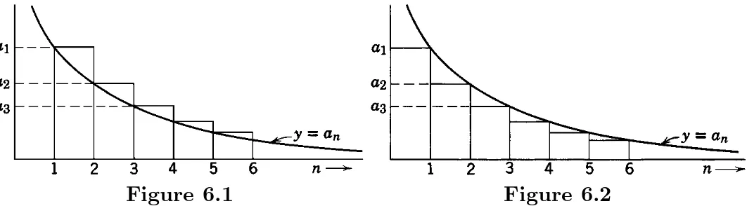
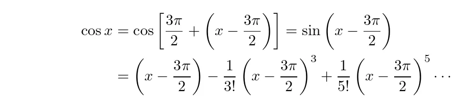
n=11/n, we consider the graph of the functiony= 1/n(similar to Figures 6.1 and 6.2) lettingnhave all values, not just integral ones. Then the values of y on the graph at n= 1,2,3,· · ·, are the terms of the series. In Figures 6.1 and 6.2, the areas of the rectangles are just the terms of the series. Notice that in Figure 6.1 the top edge of each rectangle is above the curve, so that the area of the rectangles is greater than the corresponding area under the curve. On the other hand, in Figure 6.2 the rectangles lie below the curve, so their area is less than the corresponding area under the curve. Now the areas of the rectangles are just the terms of the series, and the area under the curve is an integral ofy dnorandn. The upper limit on the integrals is∞and the lower limit could be made to correspond to any term of the series we wanted to start with. For example (see Figure 6.1), ∞
3 an dnis less than the sum of the series from
a3 on, but (see Figure 6.2) greater than the sum of the series from a4 on. If the integral is finite, then the sum of the series froma4 on is finite, that is, the series converges. Note again that the terms at the beginning of a series have nothing to do with convergence. On the other hand, if the integral is infinite, then the sum of the series froma3 on is infinite and the series diverges. Since the beginning terms are of no interest, you should simply evaluate ∞andn. (Also see Problem 16.)
Figure 6.1 Figure 6.2
Example. Test for convergence the harmonic series
(6.1) 1 +1
2 + 1 3+
1 4 +· · ·. Using the integral test, we evaluate
∞
1
n dn= lnn
∞
=∞.
(We use the symbol ln to mean a natural logarithm, that is, a logarithm to the base
Section 6 Convergence Tests for Series of Positive Terms; Absolute Convergence 13
PROBLEMS, SECTION 6
Use the integral test to find whether the following series converge or diverge. Hint and warning: Donot use lower limits on your integrals (see Problem 16).
7.
15. Use the integral test to prove the following so-called p-series test. The series ∞
Caution: Dop= 1 separately.
16. In testing P1/n2 for convergence, a student evaluates R∞
0 n
−2
dn = −n−1 |∞
0 =
0 +∞=∞and concludes (erroneously) that the series diverges. What is wrong? Hint: Consider the area under the curve in a diagram such as Figure 6.1 or 6.2. This example shows the danger of using a lower limit in the integral test.
17. Use the integral test to show thatP∞
n=0e
−n2
converges. Hint: Although you cannot evaluate the integral, you can show that it is finite (which is all that is necessary) by comparing it with R∞
e−n
dn.
C.
The Ratio Test
The integral test depends on your being able to integrateandn; this is not always easy! We consider another test which will handle many cases in which we cannot evaluate the integral. Recall that in the geometric series each term could be obtained by multiplying the one before it by the ratior, that is,an+1=ranoran+1/an=r. For other series the ratio an+1/an is not constant but depends on n; let us call the absolute value of this ratio ρn. Let us also find the limit (if there is one) of the sequence ρn as n → ∞and call this limit ρ. Thus we defineρn and ρby the
and some diverge, so we must find another test (say one of the two preceding tests). To summarize the ratio test:
(6.3) If
ρ <1, the series converges;
ρ= 1, use a different test;
ρ >1, the series diverges.
Example 1. Test for convergence the series 1 + 1 Using (6.2), we have
ρn= Sinceρ <1, the series converges.
Example 2. Test for convergence the harmonic series 1 + 1
Here the test tells us nothing and we must use some different test. A word of warning from this example: Notice that ρn =n/(n+ 1) is always less than 1. Be careful not to confuse this ratio with ρ and conclude incorrectly that this series converges. (It is actually divergent as we proved by the integral test.) Remember that ρisnot the same as the ratioρn=|an+1/an|, but is thelimit of this ratio as
n→ ∞.
PROBLEMS, SECTION 6
Use the ratio test to find whether the following series converge or diverge:
Section 6 Convergence Tests for Series of Positive Terms; Absolute Convergence 15
D.
A Special Comparison Test
This test has two parts: (a) a convergence test, and (b) a divergence test. (See Problem 37.)
(a) If∞
n=1bn is a convergent series of positive terms andan ≥0 andan/bn tends to a (finite) limit, then∞
n=1an converges. (b) If∞
n=1dn is a divergent series of positive terms and an ≥0 and an/dn tends to a limit greater than 0 (or tends to +∞), then∞
n=1an diverges.
There are really two steps in using either of these tests, namely, to decide on a comparison series, and then to compute the required limit. The first part is the most important; given a good comparison series it is a routine process to find the needed limit. The method of finding the comparison series is best shown by examples.
Example 1. Test for convergence ∞
Remember that whether a series converges or diverges depends on what the terms are as n becomes larger and larger. We are interested in the nth term as
n→ ∞. Think of n= 1010 or 10100, say; a little calculation should convince you that as n increases, 2n2 −5n+ 1 is 2n2 to quite high accuracy. Similarly, the denominator in our example is nearly 4n3for largen. By Section 9, fact 1, we see that the factor √2/4 in every term does not affect convergence. So we consider as a comparison series just
which we recognize (say by integral test) as a convergent series. Hence we use test (a) to try to show that the given series converges. We have:
lim
Since this is a finite limit, the given series converges. (With practice, you won’t need to do all this algebra! You should be able to look at the original problem and see that, for largen, the terms are essentially 1/n2, so the series converges.)
Example 2. Test for convergence
∞
n3? We can find out by comparing their logarithms since lnN andN increase or decrease together. We have ln 3n = nln 3, and lnn3 = 3 lnn. Now lnn is much smaller thann, so for largenwe havenln 3>3 lnn, and 3n > n3. (You might like to compute 1003= 106, and 3100>5×1047.) The denominator of the given series is approximatelyn5. Thus the comparison series is∞
n=23n/n5. It is easy to prove this divergent by the ratio test. Now by test (b)
lim
which is greater than zero, so the given series diverges.
PROBLEMS, SECTION 6
Use the special comparison test to find whether the following series converge or diverge.
Section 7 Alternating Series 17
7. ALTERNATING SERIES
So far we have been talking about series of positive terms (including series of abso-lute values). Now we want to consider one important case of a series whose terms have mixed signs. Analternating series is a series whose terms are alternately plus and minus; for example,
(7.1) 1−12+1
is an alternating series. We ask two questions about an alternating series. Does it converge? Does it converge absolutely (that is, when we make all signs positive)? Let us consider the second question first. In this example the series of absolute values
is the harmonic series (6.1), which diverges. We say that the series (7.1) is not absolutely convergent. Next we must ask whether (7.1) converges as it stands. If it had turned out to be absolutely convergent, we would not have to ask this question since an absolutely convergent series is also convergent (Problem 9). However, a series which is not absolutely convergent may converge or it may diverge; we must test it further. For alternating series the test is very simple:
Test for alternating series. An alternating series converges if the absolute value of the terms decreases steadily to zero, that is, if |an+1| ≤ |an| and limn→∞an= 0.
In our example 1
n+ 1 <
Test the following series for convergence.
1. 9. Prove that an absolutely convergent series P∞
n=1an is convergent. Hint: Put bn= an+|an|. Then thebnare nonnegative; we have|bn| ≤2|an|andan=bn− |an|.
10. The following alternating series are divergent (but you are not asked to prove this). Show thatan→0. Why doesn’t the alternating series test prove (incorrectly) that
8. CONDITIONALLY CONVERGENT SERIES
A series like (7.1) which converges, but does not converge absolutely, is called ditionally convergent. You have to use special care in handling conditionally con-vergent series because the positive terms alone form a dicon-vergent series and so do the negative terms alone. If you rearrange the terms, you will probably change the sum of the series, and you may even make it diverge! It is possible to rearrange the terms to make the sum any number you wish. Let us do this with the alternating harmonic series 1−12+
1 3−
1
4 +· · ·. Suppose we want to make the sum equal to 1.5. First we take enough positive terms to add to just over 1.5. The first three positive terms do this:
1 +1 3 +
1 5 = 1
8 15 >1.5.
Then we take enough negative terms to bring the partial sum back under 1.5; the one term−12 does this. Again we add positive terms until we have a little more than 1.5, and so on. Since the terms of the series are decreasing in absolute value, we are able (as we continue this process) to get partial sums just a little more or a little less than 1.5 but always nearer and nearer to 1.5. But this is what convergence of the series to the sum 1.5 means: that the partial sums should approach 1.5. You should see that we could pick in advanceany sum that we want, and rearrange the terms of this series to get it. Thus, we must not rearrange the terms of a conditionally convergent series since its convergence and its sum depend on the fact that the terms are added in a particular order.
Here is a physical example of such a series which emphasizes the care needed in applying mathematical approximations in physical problems. Coulomb’s law in electricity says that the force between two charges is equal to the product of the charges divided by the square of the distance between them (in electrostatic units; to use other units, say SI, we need only multiply by a numerical constant). Suppose there are unit positive charges atx= 0, √2, √4, √6, √8, · · ·, and unit negative charges atx= 1,√3,√5,√7,· · ·. We want to know the total force acting on the unit positive charge at x = 0 due to all the other charges. The negative charges attract the charge at x = 0 and try to pull it to the right; we call the forces exerted by them positive, since they are in the direction of the positive x
axis. The forces due to the positive charges are in the negativexdirection, and we call them negative. For example, the force due to the positive charge atx=√2 is −(1·1)/√22=−1/2. The total force on the charge atx= 0 is, then,
(8.1) F = 1−12 +1
3 − 1 4+
1 5 −
1 6 +· · ·.
Section 9 Useful Facts About Series 19
charges because there are an infinite number of them. At any stage the forces which would arise from the positive charges that are not yet in place, form a divergent series; similarly, the forces due to the unplaced negative charges form a divergent series of the opposite sign. We cannot then stop at some point and say that the rest of the series is negligible as we could in the bouncing ball problem in Section 1. But if we specify theorder in which the charges are to be placed, then the sum
S of the series is determined (S is probably different from F in (8.1) unless the charges are placed alternately). Physically this means that the value of the force as the crews proceed comes closer and closer toS, and we can use the sum of the (properly arranged)infinite series as a good approximation to the force.
9. USEFUL FACTS ABOUT SERIES
We state the following facts for reference:
1. The convergence or divergence of a series is not affected by multiplying every term of the series by the same nonzero constant. Neither is it affected by changing a finite number of terms (for example, omitting the first few terms). 2. Two convergent series ∞
n=1an and
∞
n=1bn may be added (or subtracted) term by term. (Adding “term by term” means that thenth term of the sum is an+bn.) The resulting series is convergent, and its sum is obtained by adding (subtracting) the sums of the two given series.
3. The terms of an absolutely convergent series may be rearranged in any order without affecting either the convergence or the sum. This is not true of conditionally convergent series as we have seen in Section 8.
PROBLEMS, SECTION 9
19. 1
klnn convergent?
10. POWER SERIES; INTERVAL OF CONVERGENCE
We have been discussing series whose terms were constants. Even more important and useful are series whose terms are functions of x. There are many such series, but in this chapter we shall consider series in which thenth term is a constant times
xnor a constant times (x−a)nwhereais a constant. These are calledpower series, because the terms are multiples of powers ofxor of (x−a). In later chapters we shall consider Fourier series whose terms involve sines and cosines, and other series (Legendre, Bessel, etc.) in which the terms may be polynomials or other functions.
By definition, a power series is of the form ∞
where the coefficientsan are constants. Here are some examples: 1−x2 +x
Whether a power series converges or not depends on the value of x we are considering. We often use the ratio test to find the values ofx for which a series converges. We illustrate this by testing each of the four series (10.2). Recall that in the ratio test we divide termn+ 1 by termnand take the absolute value of this ratio to getρn, and then take the limit ofρn asn→ ∞to getρ.
Example 1. For (10.2a), we have
Section 10 Power Series; Interval of Convergence 21
The series converges for ρ < 1, that is, for |x/2| <1 or |x| < 2, and it diverges for|x|>2 (see Problem 6.30). Graphically we consider the interval on the xaxis betweenx=−2 andx= 2; for any xin this interval the series (10.2a) converges. The endpoints of the interval, x= 2 and x=−2, must be considered separately. Whenx= 2, (10.2a) is
1−1 + 1−1 +· · · ,
which is divergent; whenx=−2, (10.2a) is 1 + 1 + 1 + 1 +· · ·, which is divergent. Then the interval of convergence of (10.2a) is stated as−2< x <2.
Example 2. For (10.2b) we find
ρn=
The series converges for |x| < 1. Again we must consider the endpoints of the interval of convergence, x = 1 and x = −1. For x = 1, the series (10.2b) is
4+· · ·; this is the alternating harmonic series and is convergent. For
x=−1, (10.2b) is−1−1 is divergent. Then we state the interval of convergence of (10.2b) as −1 < x≤1. Notice carefully how this differs from our result for (10.2a). Series (10.2a) did not converge at either endpoint and we used only < signs in stating its interval of convergence. Series (10.2b) converges at x = 1, so we use the sign ≤ to include
x= 1. You must always test a series at its endpoints and include the results in your statement of the interval of convergence. A series may converge at neither, either one, or both of the endpoints.
Example 3. In (10.2c), the absolute value of the nth term is|x2n−1/(2n−1)!|. To get Example 4. In (10.2d), we find
The series converges for|x+ 2|<1; that is, for−1< x+ 2<1, or−3< x <−1.
which is convergent by the alternating series test. Forx=−1, the series is
1 +√1
which is divergent by the integral test. Thus, the series converges for −3≤x <1.
PROBLEMS, SECTION 10
Find the interval of convergence of each of the following power series; be sure to investigate the endpoints of the interval in each case.
1.
The following series are not power series, but you can transform each one into a power series by a change of variable and so find out where it converges.
Section 12 Expanding Functions in Power Series 23
11. THEOREMS ABOUT POWER SERIES
We have seen that a power series∞n=0anxnconverges in some interval with center at the origin. For each value ofx(in the interval of convergence) the series has a finite sum whose value depends, of course, on the value ofx. Thus we can write the sum of the series as S(x) = ∞
n=0anxn. We see then that a power series (within its interval of convergence) defines a function of x, namelyS(x). In describing the relation of the series and the function S(x), we may say that the series converges to the functionS(x), or that the functionS(x) is represented by the series, or that the series is the power series of the function. Here we have thought of obtaining the function from a given series. We shall also (Section 12) be interested in finding a power series that converges to a given function. When we are working with power series and the functions they represent, it is useful to know the following theorems (which we state without proof; see advanced calculus texts). Power series are very useful and convenient because within their interval of convergence they can be handled much like polynomials.
1. A power series may be differentiated or integrated term by term; the resulting series converges to the derivative or integral of the function represented by the original series within the same interval of convergence as the original series (that is, not necessarily at the endpoints of the interval).
2. Two power series may be added, subtracted, or multiplied; the resultant series converges at least in the common interval of convergence. You may divide two series if the denominator series is not zero at x= 0, or if it is and the zero is canceled by the numerator [as, for example, in (sinx)/x; see (13.1)]. The resulting series will have some interval of convergence (which can be found by the ratio test or more simply by complex variable theory—see Chapter 2, Section 7).
3. One series may be substituted in another provided that the values of the substituted series are in the interval of convergence of the other series. 4. The power series of a function is unique, that is, there is just one power series
of the form∞
n=0anxn which converges to a given function.
12. EXPANDING FUNCTIONS IN POWER SERIES
Very often in applied work, it is useful to find power series that represent given functions. We illustrate one method of obtaining such series by finding the series for sinx. In this method weassume that there is such a series (see Section 14 for discussion of this point) and set out to find what the coefficients in the series must be. Thus we write
(12.1) sinx=a0+a1x+a2x2+· · ·+anxn+· · ·
and try to find numerical values of the coefficients an to make (12.1) an identity (within the interval of convergence of the series). Since the interval of convergence of a power series contains the origin, (12.1) must hold whenx= 0. If we substitute
right-hand side of the equation contain the factorx. Then to make (12.1) valid at
x= 0, we must havea0= 0. Next we differentiate (12.1) term by term to get (12.2) cosx=a1+ 2a2x+ 3a3x2+· · ·.
(This is justified by Theorem 1 of Section 11.) Again puttingx= 0, we get 1 =a1. We differentiate again, and putx= 0 to get
−sinx= 2a2+ 3·2a3x+ 4·3a4x2+· · · , 0 = 2a2.
(12.3)
Continuing the process of taking successive derivatives of (12.1) and puttingx= 0, we get
−cosx= 3·2a3+ 4·3·2a4x+· · ·, −1 = 3!a3, a3=−1
3!;
sinx= 4·3·2·a4+ 5·4·3·2a5x+· · ·, 0 =a4;
cosx= 5·4·3·2a5+· · ·, 1 = 5!a5,· · ·.
(12.4)
We substitute these values back into (12.1) and get
(12.5) sinx=x−x
3 3! +
x5 5! − · · ·.
You can probably see how to write more terms of this series without further com-putation. The sinxseries converges for allx; see Example 3, Section 10.
Series obtained in this way are called Maclaurin series or Taylor series about the origin. A Taylor series in general means a series of powers of (x−a), whereais some constant. It is found by writing (x−a) instead ofxon the right-hand side of an equation like (12.1), differentiating just as we have done, but substitutingx=a
instead ofx= 0 at each step. Let us carry out this process in general for a function
f(x). As above, we assume that there is a Taylor series forf(x), and write
f(x) =a0+a1(x−a) +a2(x−a)2+a3(x−a)3+a4(x−a)4+· · · (12.6)
+an(x−a)n+· · ·, f′
(x) =a1+ 2a2(x−a) + 3a3(x−a)2+ 4a4(x−a)3+· · · +nan(x−a)n−1+
· · ·, f′′
(x) = 2a2+ 3·2a3(x−a) + 4·3a4(x−a)2+· · · +n(n−1)an(x−a)n−2+
· · · , f′′′
(x) = 3!a3+ 4·3·2a4(x−a) +· · ·
+n(n−1)(n−2)an(x−a)n−3+· · ·, ..
.
Section 13 Techniques for Obtaining Power Series Expansions 25
[The symbolf(n)(x) means thenth derivative off(x).] We now putx=ain each equation of (12.6) and obtain
f(a) =a0, f′(a) =a1, f′′(a) = 2a2,
f′′′
(a) = 3!a3, · · · , f(n)(a) =n!an. (12.7)
[Remember thatf′
(a) means to differentiatef(x) and then putx=a;f′′
(a) means to findf′′
(x) and then put x=a, and so on.]
We can then write the Taylor series forf(x) aboutx=a:
(12.8) f(x) =f(a) + (x−a)f′ (a) + 1
2!(x−a) 2f′′
(a) +· · ·+ 1
n!(x−a)
nf(n)(a) + · · ·.
The Maclaurin series for f(x) is the Taylor series about the origin. Putting
a= 0 in (12.8), we obtain the Maclaurin series forf(x):
(12.9) f(x) =f(0) +xf′ (0) +x
2 2!f
′′ (0) +x
3 3!f
′′′
(0) +· · ·+x n
n!f
(n)(0) + · · · .
We have written this in general because it is sometimes convenient to have the formulas for the coefficients. However, finding the higher order derivatives in (12.9) for any but the simplest functions is unnecessarily complicated (try it for, say,etanx). In Section 13, we shall discuss much easier ways of getting Maclaurin and Taylor series by combining a few basic series. Meanwhile, you should verify (Problem 1, below) the basic series (13.1) to (13.5) and memorize them.
PROBLEMS, SECTION 12
1. By the method used to obtain (12.5) [which is the series (13.1) below], verify each of the other series (13.2) to (13.5) below.
13. TECHNIQUES FOR OBTAINING POWER SERIES EXPANSIONS
There are often simpler ways for finding the power series of a function than the successive differentiation process in Section 12. Theorem 4 in Section 11 tells us that for a given function there isjust one power series, that is, just one series of the form ∞
convergent for
(binomial series; pis any real number, positive or negative and pn is called a binomial coefficient—see method C below.)
When we use a series to approximate a function, we may want only the first few terms, but in derivations, we may want the formula for the general term so that we can write the series in summation form. Let’s look at some methods of obtaining either or both of these results.
A.
Multiplying a Series by a Polynomial or by Another Series
Example 1. To find the series for (x+ 1) sinx, we multiply (x+ 1) times the series (13.1)