1 Python code for Artificial Intelligence: Foundations of Computational Agents

(1)

1

Python code for Artificial

Intelligence: Foundations of

Computational Agents

David L. Poole and Alan K. Mackworth

Version 0.7.6 of August 20, 2018.

http://aipython.org

http://artint.info

©David L Poole and Alan K Mackworth 2017.

All code is licensed under a Creative Commons

Attribution-NonCommercial-ShareAlike 4.0 International License. See:

http://creativecommons.org/licenses/

by-nc-sa/4.0/deed.en US

This document and all the code can be downloaded from

http://artint.info/AIPython/

_{or from}

http://aipython.org

(2)

(3)

Chapter 1 Python for Artificial Intelligence

1.1 Why Python?

We use Python because Python programs can be close to pseudo-code. It is

designed for humans to read.

Python is reasonably efficient. Efficiency is usually not a problem for small

examples. If your Python code is not efficient enough, a general procedure

to improve it is to find out what is taking most the time, and implement just

that part more efficiently in some level language. Most of these

lower-level languages interoperate with Python nicely. This will result in much less

programming and more efficient code (because you will have more time to

optimize) than writing everything in a low-level language. You will not have

to do that for the code here if you are using it for course projects.

1.2 Getting Python

You need Python 3 (

http://python.org/

) and matplotlib (

http://matplotlib.

org/

_{) that runs with Python 3. This code is}

not

compatible with Python 2 (e.g.,

with Python 2.7).

Download and istall the latest Python 3 release from

http://python.org/

.

This should also install

pip

3. You can install matplotlib using

pip3 install matplotlib

in a terminal shell (not in Python). That should “just work”. If not, try using

pip

_{instead of}

pip3

_.

(8)

To upgrade matplotlib to the latest version (which you should do if you

install a new version of Python) do:

pip3 install --upgrade matplotlib

We recommend using the enhanced interactive python

ipython

(

http://

ipython.org/

). To install ipython after you have installed python do:

pip3 install ipython

1.3 Running Python

We assume that everything is done with an interactive Python shell. You can

either do this with an IDE, such as IDLE that comes with standard Python

distributions, or just running ipython3 (or perhaps just ipython) from a shell.

Here we describe the most simple version that uses no IDE. If you

down-load the zip file, and cd to the “

aipython

” folder where the .py files are, you

should be able to do the following, with user input following

:

. The first

ipython3 command is in the operating system shell (note that the

-i

_is

impor-tant to enter interactive mode):

$ ipython3 -i searchGeneric.py

Python 3.6.5 (v3.6.5:f59c0932b4, Mar 28 2018, 05:52:31)

Type 'copyright', 'credits' or 'license' for more information

IPython 6.2.1 -- An enhanced Interactive Python. Type '?' for help.

Testing problem 1:

7 paths have been expanded and 4 paths remain in the frontier

Path found: a --> b --> c --> d --> g

Passed unit test

In [1]: searcher2 = AStarSearcher(searchProblem.acyclic_delivery_problem) #A*

In [2]: searcher2.search()

# find first path

16 paths have been expanded and 5 paths remain in the frontier

Out[2]: o103 --> o109 --> o119 --> o123 --> r123

In [3]: searcher2.search()

# find next path

21 paths have been expanded and 6 paths remain in the frontier

Out[3]: o103 --> b3 --> b4 --> o109 --> o119 --> o123 --> r123

In [4]: searcher2.search()

# find next path

28 paths have been expanded and 5 paths remain in the frontier

Out[4]: o103 --> b3 --> b1 --> b2 --> b4 --> o109 --> o119 --> o123 --> r123

In [5]: searcher2.search()

# find next path

(9)

1.4. Pitfalls

9 In [6]:

You can then interact at the last prompt.

There are many textbooks for Python. The best source of information about

python is

https://www.python.org/

. We will be using Python 3; please

down-load the latest release. The documentation is at

https://docs.python.org/3/

.

The rest of this chapter is about what is special about the code for AI tools.

We will only use the Standard Python Library and matplotlib. All of the

exer-cises can be done (and should be done) without using other libraries; the aim

is for you to spend your time thinking about how to solve the problem rather

than searching for pre-existing solutions.

1.4 Pitfalls

It is important to know when side effects occur. Often AI programs consider

what would happen or what may have happened. In many such cases, we

don’t want side effects. When an agent acts in the world, side effects are

ap-propriate.

In Python, you need to be careful to understand side effects. For example,

the inexpensive function to add an element to a list, namely

append

, changes

the list. In a functional language like Lisp, adding a new element to a list,

without changing the original list, is a cheap operation. For example if

x

is a

list containing

n

elements, adding an extra element to the list in Python (using

append

) is fast, but it has the side effect of changing the list

x

. To construct a

new list that contains the elements of

x

plus a new element, without changing

the value of

x

, entails copying the list, or using a different representation for

lists. In the searching code, we will use a different representation for lists for

this reason.

1.5 Features of Python

1.5.1 Lists, Tuples, Sets, Dictionaries and Comprehensions

We make extensive uses of lists, tuples, sets and dictionaries (dicts). See

https://docs.python.org/3/library/stdtypes.html

One of the nice features of Python is the use of list comprehensions (and

also tuple, set and dictionary comprehensions).

(

fe

for

e

in

iter

if

cond

)

(10)

is an expression that evaluates to either True or False for each

e

, and

fe

is an

expression that will be evaluated for each value of

e

for which

cond

returns

True

.

The result can go in a list or used in another iteration, or can be called

directly using

. The procedure

takes an iterator returns the next

el-ement (advancing the iterator) and raises a StopIteration exception if there is

no next element. The following shows a simple example, where user input is

prepended with

>>>

>>> [e*e for e in range(20) if e%2==0]

[0, 4, 16, 36, 64, 100, 144, 196, 256, 324]

>>> a = (e*e for e in range(20) if e%2==0)

>>> next(a)

0 >>> next(a)

4 >>> next(a)

16 >>> list(a)

[36, 64, 100, 144, 196, 256, 324]

>>> next(a)

Traceback (most recent call last):

File "<stdin>", line 1, in <module>

StopIteration

Notice how

list

(

a

)

continued on the enumeration, and got to the end of it.

Comprehensions can also be used for dictionaries. The following code

cre-ates an index for list

a

:

>>> a = ["a","f","bar","b","a","aaaaa"]

>>> ind = {a[i]:i for i in range(len(a))}

>>> ind

{'a': 4, 'f': 1, 'bar': 2, 'b': 3, 'aaaaa': 5}

>>> ind['b']

3 which means that

'b'

is the 3rd element of the list.

The assignment of

ind

could have also be written as:

>>> ind = {val:i for (i,val) in enumerate(a)}

where

enumerate

returns an iterator of

(

index

,

value

)

pairs.

1.5.2 Functions as first-class objects

(11)

1.5. Features of Python

11 called

, not the value of the variable when the function was defined (this is called

“late binding”). This means if you want to use the value a variable has when

the function is created, you need to save the current value of that variable.

Whereas Python uses “late binding” by default, the alternative that newcomers

often expect is “early binding”, where a function uses the value a variable had

when the function was defined, can be easily implemented.

Consider the following programs designed to create a list of 5 functions,

where the

i

th function in the list is meant to add

i

to its argument:

1

pythonDemo.py — Some tricky examples

11 fun_list1 = [] 12 for i in range(5): 13 def fun1(e): 14 return e+i

15 fun_list1.append(fun1) 16

17 fun_list2 = [] 18 for i in range(5): 19 def fun2(e,iv=i): 20 return e+iv

21 fun_list2.append(fun2) 22

23 fun_list3 = [lambda e: e+i for i in range(5)] 24

25 fun_list4 = [lambda e,iv=i: e+iv for i in range(5)] 26

27 i=56

Try to predict, and then test to see the output, of the output of the following

calls, remembering that the function uses the latest value of any variable that

is not bound in the function call:

pythonDemo.py — (continued)

29 # in Shell do

30 ## ipython -i pythonDemo.py

31 # Try these (copy text after the comment symbol and paste in the Python prompt): 32 # print([f(10) for f in fun_list1])

33 # print([f(10) for f in fun_list2]) 34 # print([f(10) for f in fun_list3]) 35 # print([f(10) for f in fun_list4])

In the first for-loop, the function

fun

uses

i

, whose value is the last value it was

assigned. In the second loop, the function

fun

2 uses

iv

. There is a separate

iv

variable for each function, and its value is the value of

i

when the function was

defined. Thus

fun

1 uses late binding, and

fun

2 uses early binding.

fun list

3 and

fun list

4 are equivalent to the first two (except

fun list

4 uses a different

i

variable).

1_{Numbered lines are Python code available in the code-directory,}_aipython_{. The name of}

(12)

One of the advantages of using the embedded definitions (as in

fun

1 and

fun

2 above) over the lambda is that is it possible to add a

doc

string, which

is the standard for documenting functions in Python, to the embedded

defini-tions.

1.5.3 Generators and Coroutines

Python has generators which can be used for a form of coroutines.

The

yield

command returns a value that is obtained with

. It is typically

used to enumerate the values for a

for

loop or in generators.

A version of the built-in

range

, with 2 or 3 arguments (and positive steps)

can be implemented as:

37 def myrange(start, stop, step=1):

38 """enumerates the values from start in steps of size step that are 39 less than stop.

40 """

41 assert step>0, "only positive steps implemented in myrange" 42 i = start

43 while i<stop:

44 yield i

45 i += step

46

47 print("myrange(2,30,3):",list(myrange(2,30,3)))

Note that the built-in

range

is unconventional in how it handles a single

ar-gument, as the single argument acts as the second argument of the function.

Note also that the built-in range also allows for indexing (e.g.,

range

(

2, 30, 3

)[

2 ]

returns 8), which the above implementation does not. However

myrange

also

works for floats, which the built-in range does not.

Exercise 1.1

Implement a version ofmyrangethat acts like the built-in version when there is a single argument. (Hint: make the second argument have a default value that can be recognized in the function.)

Yield can be used to generate the same sequence of values as in the example

of Section 1.5.1:

49 def ga(n):

50 """generates square of even nonnegative integers less than n""" 51 for e in range(n):

52 if e%2==0:

53 yield e*e

54 a = ga(20)

(13)

1.6. Useful Libraries

13 It is straightforward to write a version of the built-in

enumerate

. Let’s call it

myenumerate

:

56 def myenumerate(enum):

57 for i in range(len(enum)):

58 yield i,enum[i]

Exercise 1.2

Write a version ofenumeratewhere the only iteration is “for val in enum”. Hint: keep track of the index.

1.6 Useful Libraries

1.6.1 Timing Code

In order to compare algorithms, we often want to compute how long a program

takes; this is called the

runtime

of the program. The most straightforward way

to compute runtime is to use

time

.

perf counter

()

, as in:

import time

start_time = time.perf_counter()

compute_for_a_while()

end_time = time.perf_counter()

print("Time:", end_time - start_time, "seconds")

If this time is very small (say less than 0.2 second), it is probably very

inac-curate, and it may be better to run your code many times to get a more

accu-rate count. For this you can use

timeit

(

https://docs.python.org/3/library/

timeit.html

). To use timeit to time the call to

foo

.

bar

(

aaa

)

use:

import timeit

time = timeit.timeit("foo.bar(aaa)",

setup="from main import foo,aaa", number=100)

The setup is needed so that Python can find the meaning of the names in the

string that is called. This returns the number of seconds to execute

foo

.

bar

(

aaa

)

100 times. The variable

number

should be set so that the runtime is at least 0.2

seconds.

You should not trust a single measurement as that can be confounded by

interference from other processes.

timeit

.

repeat

can be used for running

timit

a few (say 3) times. Usually the minimum time is the one to report, but you

should be explicit and explain what you are reporting.

1.6.2 Plotting: Matplotlib

The standard plotting for Python is matplotlib (

http://matplotlib.org/

_{). We}

(14)

60 import matplotlib.pyplot as plt 61

62 def myplot(min,max,step,fun1,fun2): 63 plt.ion() # make it interactive 64 plt.xlabel("The x axis")

65 plt.ylabel("The y axis")

66 plt.xscale('linear') # Makes a 'log' or 'linear' scale 67 xvalues = range(min,max,step)

68 plt.plot(xvalues,[fun1(x) for x in xvalues], 69 label="The first fun")

70 plt.plot(xvalues,[fun2(x) for x in xvalues], linestyle='--',color='k', 71 label=fun2.__doc__) # use the doc string of the function 72 plt.legend(loc="upper right") # display the legend

73

74 def slin(x): 75 """y=2x+7""" 76 return 2*x+7 77 def sqfun(x):

78 """y=(x-40)ˆ2/10-20""" 79 return (x-40)**2/10-20 80

81 # Try the following:

82 # from pythonDemo import myplot, slin, sqfun 83 # import matplotlib.pyplot as plt

84 # myplot(0,100,1,slin,sqfun) 85 # plt.legend(loc="best") 86 # import math

87 # plt.plot([41+40*math.cos(th/10) for th in range(50)], 88 # [100+100*math.sin(th/10) for th in range(50)]) 89 # plt.text(40,100,"ellipse?")

90 # plt.xscale('log')

At the end of the code are some commented-out commands you should try in

interactive mode. Cut from the file and paste into Python (and remember to

remove the comments symbol and leading space).

1.7 Utilities

1.7.1 Display

In this distribution, to keep things simple and to only use standard Python, we

use a text-oriented tracing of the code. A graphical depiction of the code could

override the definition of

display

(but we leave it as a project).

The method

self

.

display

is used to trace the program. Any call

(15)

1.7. Utilities

15 where the level is less than or equal to the value for

max display level

will be

printed. The

to print

. . . can be anything that is accepted by the built-in

print

(including any keyword arguments).

The definition of

display

is:

display.py — AIFCA utilities

11 class Displayable(object): 12 """Class that uses 'display'.

13 The amount of detail is controlled by max_display_level 14 """

15 max_display_level = 1 # can be overridden in subclasses 16

17 def display(self,level,*args,**nargs):

18 """print the arguments if level is less than or equal to the 19 current max_display_level.

20 level is an integer.

21 the other arguments are whatever arguments print can take. 22 """

23 if level <= self.max_display_level:

24 print(*args, **nargs) ##if error you are using Python2 not Python3

Note that

args

gets a tuple of the positional arguments, and

nargs

gets a

dictio-nary of the keyword arguments). This will not work in Python 2, and will give

an error.

Any class that wants to use

display

can be made a subclass of

Displayable

.

To change the maximum display level to say 3, for a class do:

Classname

.

max display level

=

3 which will make calls to

display

in that class print when the value of

level

is less

than-or-equal to 3. The default display level is 1. It can also be changed for

individual objects (the object value overrides the class value).

The value of

max display level

by convention is:

0 display nothing

1 display solutions (nothing that happens repeatedly)

2 also display the values as they change (little detail through a loop)

3 also display more details

4 and above

even more detail

In order to implement more sophisticated visualizations of the algorithm,

we add a

visualize

“decorator” to the methods to be visualized. The following

code ignores the decorator:

display.py — (continued)

(16)

27 """A decorator for algorithms that do interactive visualization. 28 Ignored here.

29 """

30 return func

1.7.2 Argmax

Python has a built-in

max

function that takes a generator (or a list or set) and

re-turns the maximum value. The

argmax

method returns the index of an element

that has the maximum value. If there are multiple elements with the maximum

value, one if the indexes to that value is returned at random. This assumes a

generator of

(

element

,

value

)

pairs, as for example is generated by the built-in

enumerate

.

utilities.py — AIPython useful utilities

11 import random 12

13 def argmax(gen):

14 """gen is a generator of (element,value) pairs, where value is a real. 15 argmax returns an element with maximal value.

16 If there are multiple elements with the max value, one is returned at random. 17 """

18 maxv = float('-Infinity') # negative infinity 19 maxvals = [] # list of maximal elements 20 for (e,v) in gen:

21 if v>maxv:

22 maxvals,maxv = [e], v

23 elif v==maxv:

24 maxvals.append(e)

25 return random.choice(maxvals) 26

27 # Try:

28 # argmax(enumerate([1,6,3,77,3,55,23]))

Exercise 1.3

Change argmax to have an optinal argument that specifies whether you want the “first”, “last” or a “random” index of the maximum value returned. If you want the first or the last, you don’t need to keep a list of the maximum elements.

1.7.3 Probability

For many of the simulations, we want to make a variable True with some

prob-ability.

flip

(

p

)

returns True with probability

p

, and otherwise returns False.

utilities.py — (continued)

30 def flip(prob):

(17)

1.8. Testing Code

17

1.7.4 Dictionary Union

The function

dict union

(

d

1,

d

2 )

returns the union of dictionaries

d

1 and

d

2. If

the values for the keys conflict, the values in

d

2 are used. This is similar to

dict

(

d

1,

∗ ∗

d

2 )

, but that only works when the keys of

d

2 are strings.

34 def dict_union(d1,d2):

35 """returns a dictionary that contains the keys of d1 and d2. 36 The value for each key that is in d2 is the value from d2, 37 otherwise it is the value from d1.

38 This does not have side effects. 39 """

40 d = dict(d1) # copy d1 41 d.update(d2)

42 return d

1.8 Testing Code

It is important to test code early and test it often. We include a simple form of

unit tests

. The value of the current module is in

name

and if the module is

run at the top-level, it’s value is

"main"

. See

https://docs.python.org/3/

library/ main .html

_.

The following code tests

argmax

and

dict_union

, but only when if

utilities

is loaded in the top-level. If it is loaded in a module the test code is not run.

In your code you should do more substantial testing than we do here, in

particular testing the boundary cases.

44 def test():

45 """Test part of utilities"""

46 assert argmax(enumerate([1,6,55,3,55,23])) in [2,4]

47 assert dict_union({1:4, 2:5, 3:4},{5:7, 2:9}) == {1:4, 2:9, 3:4, 5:7} 48 print("Passed unit test in utilities")

49

50 if __name__ == "__main__":

(18)

(19)

Chapter 2 Agents and Control

This implements the controllers described in Chapter 2.

In this version the higher-levels call the lower-levels. A more

sophisti-cated version may have them run concurrently (either as coroutines or in

paral-lel). The higher-levels calling the lower-level works in simulated environments

when there is a single agent, and where the lower-level are written to make sure

they return (and don’t go on forever), and the higher level doesn’t take too long

(as the lower-levels will wait until called again).

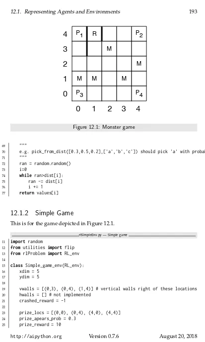
2.1 Representing Agents and Environments

An agent observes the world, and carries out actions in the environment, it also

has an internal state that it updates. The environment takes in actions of the

agents, updates it internal state and returns the percepts.

In this implementation, the state of the agent and the state of the

environ-ment are represented using standard Python variables, which are updated as

the state changes. The percepts and the actions are represented as

variable-value dictionaries.

An agent implements the

go

(

n

)

method, where

n

is an integer. This means

that the agent should run for

n

time steps.

In the following code

raise NotImplementedError()

is a way to specify

an abstract method that needs to be overidden in any implemented agent or

environment.

agents.py — Agent and Controllers

11 import random 12

(20)

15 """set up the agent"""

16 self.env=env

17

18 def go(self,n):

19 """acts for n time steps"""

20 raise NotImplementedError("go") # abstract method

The environment implements a

do

(

action

)

method where

action

is a

variable-value dictionary. This returns a percept, which is also a variable-variable-value

dictio-nary. The use of dictionaries allows for structured actions and percepts.

Note that

Environment

is a subclass of

Displayable

so that it can use the

display

method described in Section 1.7.1.

agents.py — (continued)

22 from utilities import Displayable 23 class Environment(Displayable): 24 def initial_percepts(self):

25 """returns the initial percepts for the agent"""

26 raise NotImplementedError("initial_percepts") # abstract method 27

28 def do(self,action):

29 """does the action in the environment 30 returns the next percept """

31 raise NotImplementedError("do") # abstract method

2.2 Paper buying agent and environment

To run the demo, in folder ”

aipython

”, load ”

agents.py

”, using e.g.,

ipython

-i

agents.py

, and copy and paste the commented-out

commands at the bottom of that file. This requires Python 3 with

matplotlib

_.

This is an implementation of the paper buying example.

2.2.1 The Environment

The environment state is given in terms of the

time

and the amount of paper in

stock

. It also remembers the in-stock history and the price history. The percepts

are the price and the amount of paper in stock. The action of the agent is the

number to buy.

Here we assume that the prices are obtained from the

prices

list plus a

ran-dom integer in range

[

0,

max price addon

)

plus a linear ”inflation”. The agent

cannot access the price model; it just observes the prices and the amount in

stock.

(21)

2.2. Paper buying agent and environment

21

41 max_price_addon = 20 # maximum of random value added to get price 42

43 def __init__(self):

44 """paper buying agent"""

45 self.time=0

46 self.stock=20

47 self.stock_history = [] # memory of the stock history 48 self.price_history = [] # memory of the price history 49

50 def initial_percepts(self): 51 """return initial percepts"""

52 self.stock_history.append(self.stock)

53 price = self.prices[0]+random.randrange(self.max_price_addon) 54 self.price_history.append(price)

55 return {'price': price,

56 'instock': self.stock}

57

58 def do(self, action):

59 """does action (buy) and returns percepts (price and instock)""" 60 used = pick_from_dist({6:0.1, 5:0.1, 4:0.2, 3:0.3, 2:0.2, 1:0.1}) 61 bought = action['buy']

62 self.stock = self.stock+bought-used 63 self.stock_history.append(self.stock)

64 self.time += 1

65 price = (self.prices[self.time%len(self.prices)] # repeating pattern 66 +random.randrange(self.max_price_addon) # plus randomness

67 +self.time//2) # plus inflation

68 self.price_history.append(price) 69 return {'price': price,

70 'instock': self.stock}

The

pick from dist

method takes in a

item

:

probability

dictionary, and returns

one of the items in proportion to its probability.

72 def pick_from_dist(item_prob_dist):

73 """ returns a value from a distribution.

74 item_prob_dist is an item:probability dictionary, where the 75 probabilities sum to 1.

76 returns an item chosen in proportion to its probability 77 """

78 ranreal = random.random()

(22)

81 return it

82 else:

83 ranreal -= prob

84 raise RuntimeError(str(item_prob_dist)+" is not a probability distribution")

2.2.2 The Agent

The agent does not have access to the price model but can only observe the

current price and the amount in stock. It has to decide how much to buy.

The belief state of the agent is an estimate of the average price of the paper,

and the total amount of money the agent has spent.

86 class TP_agent(Agent): 87 def __init__(self, env):

88 self.env = env

89 self.spent = 0

90 percepts = env.initial_percepts()

91 self.ave = self.last_price = percepts['price'] 92 self.instock = percepts['instock']

93

94 def go(self, n):

95 """go for n time steps 96 """

97 for i in range(n):

98 if self.last_price < 0.9*self.ave and self.instock < 60:

99 tobuy = 48

100 elif self.instock < 12:

101 tobuy = 12

102 else:

103 tobuy = 0

104 self.spent += tobuy*self.last_price 105 percepts = env.do({'buy': tobuy}) 106 self.last_price = percepts['price']

107 self.ave = self.ave+(self.last_price-self.ave)*0.05 108 self.instock = percepts['instock']

Set up an environment and an agent. Uncomment the last lines to run the agent

for 90 steps, and determine the average amount spent.

110 env = TP_env() 111 ag = TP_agent(env) 112 #ag.go(90)

113 #ag.spent/env.time ## average spent per time period

2.2.3 Plotting

(23)

2.3. Hierarchical Controller

23

117 class Plot_prices(object):

118 """Set up the plot for history of price and number in stock""" 119 def __init__(self, ag,env):

120 self.ag = ag

121 self.env = env

122 plt.ion()

123 plt.xlabel("Time")

124 plt.ylabel("Number in stock. Price.")

125

126 def plot_run(self):

127 """plot history of price and instock""" 128 num = len(env.stock_history)

129 plt.plot(range(num),env.stock_history,label="In stock") 130 plt.plot(range(num),env.price_history,label="Price") 131 #plt.legend(loc="upper left")

132 plt.draw()

133

134 # pl = Plot_prices(ag,env) 135 # ag.go(90); pl.plot_run()

2.3 Hierarchical Controller

To run the hierarchical controller, in folder ”

aipython

”, load

”

agentTop.py

_{”, using e.g.,}

ipython -i agentTop.py

_{, and copy and}

paste the commands near the bottom of that file. This requires Python

3 with

matplotlib

.

In this implementation, each layer, including the top layer, implements the

en-vironment class, because each layer is seen as an enen-vironment from the layer

above.

We arbitrarily divide the environment and the body, so that the

environ-ment just defines the walls, and the body includes everything to do with the

agent. Note that the named locations are part of the (top-level of the) agent,

not part of the environment, although they could have been.

2.3.1 Environment

The environment defines the walls.

agentEnv.py — Agent environment

11 import math

12 from agents import Environment 13

(24)

15 def __init__(self,walls = {}):

16 """walls is a set of line segments

17 where each line segment is of the form ((x0,y0),(x1,y1)) 18 """

19 self.walls = walls

2.3.2 Body

The body defines everything about the agent body.

agentEnv.py — (continued)

21 import math

22 from agents import Environment 23 import matplotlib.pyplot as plt 24 import time

25

26 class Rob_body(Environment):

27 def __init__(self, env, init_pos=(0,0,90)): 28 """ env is the current environment

29 init_pos is a triple of (x-position, y-position, direction) 30 direction is in degrees; 0 is to right, 90 is straight-up, etc 31 """

32 self.env = env

33 self.rob_x, self.rob_y, self.rob_dir = init_pos 34 self.turning_angle = 18 # degrees that a left makes 35 self.whisker_length = 6 # length of the whisker

36 self.whisker_angle = 30 # angle of whisker relative to robot 37 self.crashed = False

38 # The following control how it is plotted

39 self.plotting = True # whether the trace is being plotted

40 self.sleep_time = 0.05 # time between actions (for real-time plotting) 41 # The following are data structures maintained:

42 self.history = [(self.rob_x, self.rob_y)] # history of (x,y) positions 43 self.wall_history = [] # history of hitting the wall

44

45 def percepts(self):

46 return {'rob_x_pos':self.rob_x, 'rob_y_pos':self.rob_y,

47 'rob_dir':self.rob_dir, 'whisker':self.whisker() , 'crashed':self.crashed} 48 initial_percepts = percepts # use percept function for initial percepts too

49

50 def do(self,action):

51 """ action is {'steer':direction}

52 direction is 'left', 'right' or 'straight' 53 """

54 if self.crashed:

55 return self.percepts() 56 direction = action['steer']

(25)

2.3. Hierarchical Controller

25

60 rob_y_new = self.rob_y + math.sin(self.rob_dir*math.pi/180) 61 path = ((self.rob_x,self.rob_y),(rob_x_new,rob_y_new))

62 if any(line_segments_intersect(path,wall) for wall in self.env.walls):

63 self.crashed = True

64 if self.plotting:

65 plt.plot([self.rob_x],[self.rob_y],"r*",markersize=20.0)

66 plt.draw()

67 self.rob_x, self.rob_y = rob_x_new, rob_y_new 68 self.history.append((self.rob_x, self.rob_y)) 69 if self.plotting and not self.crashed:

70 plt.plot([self.rob_x],[self.rob_y],"go")

71 plt.draw()

72 plt.pause(self.sleep_time) 73 return self.percepts()

This detects if the whisker and the wall intersect. It’s value is returned as a

percept.

agentEnv.py — (continued)

75 def whisker(self):

76 """returns true whenever the whisker sensor intersects with a wall 77 """

78 whisk_ang_world = (self.rob_dir-self.whisker_angle)*math.pi/180 79 # angle in radians in world coordinates

80 wx = self.rob_x + self.whisker_length * math.cos(whisk_ang_world) 81 wy = self.rob_y + self.whisker_length * math.sin(whisk_ang_world) 82 whisker_line = ((self.rob_x,self.rob_y),(wx,wy))

83 hit = any(line_segments_intersect(whisker_line,wall)

84 for wall in self.env.walls)

85 if hit:

93 """returns true if the line segments, linea and lineb intersect. 94 A line segment is represented as a pair of points.

95 A point is represented as a (x,y) pair. 96 """

97 ((x0a,y0a),(x1a,y1a)) = linea 98 ((x0b,y0b),(x1b,y1b)) = lineb 99 da, db = x1a-x0a, x1b-x0b 100 ea, eb = y1a-y0a, y1b-y0b 101 denom = db*ea-eb*da

102 if denom==0: # line segments are parallel 103 return False

104 cb = (da*(y0b-y0a)-ea*(x0b-x0a))/denom # position along line b 105 if cb<0 or cb>1:

(26)

107 ca = (db*(y0b-y0a)-eb*(x0b-x0a))/denom # position along line a 108 return 0<=ca<=1

109

110 # Test cases:

111 # assert line_segments_intersect(((0,0),(1,1)),((1,0),(0,1)))

112 # assert not line_segments_intersect(((0,0),(1,1)),((1,0),(0.6,0.4))) 113 # assert line_segments_intersect(((0,0),(1,1)),((1,0),(0.4,0.6)))

2.3.3 Middle Layer

The middle layer acts like both a controller (for the environment layer) and an

environment for the upper layer. It has to tell the environment how to steer.

Thus it calls

env

.

do

(·)

. It also is told the position to go to and the timeout. Thus

it also has to implement

do

(·)

.

agentMiddle.py — Middle Layer

11 from agents import Environment 12 import math

13

14 class Rob_middle_layer(Environment): 15 def __init__(self,env):

16 self.env=env

17 self.percepts = env.initial_percepts()

18 self.straight_angle = 11 # angle that is close enough to straight ahead 19 self.close_threshold = 2 # distance that is close enough to arrived

20 self.close_threshold_squared = self.close_threshold**2 # just compute it once 21

22 def initial_percepts(self): 23 return {}

24

25 def do(self, action):

26 """action is {'go_to':target_pos,'timeout':timeout} 27 target_pos is (x,y) pair

28 timeout is the number of steps to try

29 returns {'arrived':True} when arrived is true 30 or {'arrived':False} if it reached the timeout 31 """

32 if 'timeout' in action:

33 remaining = action['timeout']

34 else:

35 remaining = -1 # will never reach 0 36 target_pos = action['go_to']

37 arrived = self.close_enough(target_pos) 38 while not arrived and remaining != 0:

39 self.percepts = self.env.do({"steer":self.steer(target_pos)})

40 remaining -= 1

(27)

2.3. Hierarchical Controller

27 This determines how to steer depending on whether the goal is to the right or

the left of where the robot is facing.

agentMiddle.py — (continued)

44 def steer(self,target_pos): 45 if self.percepts['whisker']:

46 self.display(3,'whisker on', self.percepts) 47 return "left"

48 else:

49 gx,gy = target_pos

50 rx,ry = self.percepts['rob_x_pos'],self.percepts['rob_y_pos'] 51 goal_dir = math.acos((gx-rx)/math.sqrt((gx-rx)*(gx-rx)

52 +(gy-ry)*(gy-ry)))*180/math.pi

53 if ry>gy:

54 goal_dir = -goal_dir

55 goal_from_rob = (goal_dir - self.percepts['rob_dir']+540)%360-180 56 assert -180 < goal_from_rob <= 180

57 if goal_from_rob > self.straight_angle: 58 return "left"

59 elif goal_from_rob < -self.straight_angle: 60 return "right"

61 else:

62 return "straight" 63

64 def close_enough(self,target_pos): 65 gx,gy = target_pos

66 rx,ry = self.percepts['rob_x_pos'],self.percepts['rob_y_pos'] 67 return (gx-rx)**2 + (gy-ry)**2 <= self.close_threshold_squared

2.3.4 Top Layer

The top layer treats the middle layer as its environment. Note that the top layer

is an environment for us to tell it what to visit.

agentTop.py — Top Layer

11 from agentMiddle import Rob_middle_layer 12 from agents import Environment

13

14 class Rob_top_layer(Environment):

15 def __init__(self, middle, timeout=200, locations = {'mail':(-5,10),

16 'o103':(50,10), 'o109':(100,10),'storage':(101,51)} ):

17 """middle is the middle layer

18 timeout is the number of steps the middle layer goes before giving up 19 locations is a loc:pos dictionary

20 where loc is a named location, and pos is an (x,y) position. 21 """

22 self.middle = middle

23 self.timeout = timeout # number of steps before the middle layer should give up 24 self.locations = locations

(28)

26 def do(self,plan): 27 """carry out actions.

28 actions is of the form {'visit':list_of_locations} 29 It visits the locations in turn.

30 """

31 to_do = plan['visit'] 32 for loc in to_do:

33 position = self.locations[loc]

34 arrived = self.middle.do({'go_to':position, 'timeout':self.timeout}) 35 self.display(1,"Arrived at",loc,arrived)

2.3.5 Plotting

The following is used to plot the locations, the walls and (eventually) the

move-ment of the robot. It can either plot the movemove-ment if the robot as it is

go-ing (with the default

env

.

plotting

=

True

), or not plot it as it is going (setting

env

.

plotting

=

False

; in this case the trace can be plotted using

pl

.

plot run

()

).

agentTop.py — (continued)

39 class Plot_env(object):

40 def __init__(self, body,top): 41 """sets up the plot 42 """

43 self.body = body

44 plt.ion()

45 plt.clf()

46 plt.axes().set_aspect('equal') 47 for wall in body.env.walls:

48 ((x0,y0),(x1,y1)) = wall

49 plt.plot([x0,x1],[y0,y1],"-k",linewidth=3) 50 for loc in top.locations:

51 (x,y) = top.locations[loc] 52 plt.plot([x],[y],"k<")

53 plt.text(x+1.0,y+0.5,loc) # print the label above and to the right 54 plt.plot([body.rob_x],[body.rob_y],"go")

55 plt.draw()

56

57 def plot_run(self):

58 """plots the history after the agent has finished. 59 This is typically only used if body.plotting==False 60 """

61 xs,ys = zip(*self.body.history) 62 plt.plot(xs,ys,"go")

63 wxs,wys = zip(*self.body.wall_history) 64 plt.plot(wxs,wys,"ro")

65 #plt.draw()

(29)

2.3. Hierarchical Controller

29

67 from agentEnv import Rob_body, Rob_env 68

69 env = Rob_env({((20,0),(30,20)), ((70,-5),(70,25))}) 70 body = Rob_body(env)

71 middle = Rob_middle_layer(body) 72 top = Rob_top_layer(middle) 73

74 # try:

75 # pl=Plot_env(body,top)

76 # top.do({'visit':['o109','storage','o109','o103']}) 77 # You can directly control the middle layer:

78 # middle.do({'go_to':(30,-10), 'timeout':200}) 79 # Can you make it crash?

Exercise 2.1

The following code implements a robot trap. Write a controller that can escape the “trap” and get to the goal. See textbook for hints.

81 # Robot Trap for which the current controller cannot escape:

82 trap_env = Rob_env({((10,-21),(10,0)), ((10,10),(10,31)), ((30,-10),(30,0)), 83 ((30,10),(30,20)), ((50,-21),(50,31)), ((10,-21),(50,-21)), 84 ((10,0),(30,0)), ((10,10),(30,10)), ((10,31),(50,31))}) 85 trap_body = Rob_body(trap_env,init_pos=(-1,0,90))

86 trap_middle = Rob_middle_layer(trap_body)

87 trap_top = Rob_top_layer(trap_middle,locations={'goal':(71,0)}) 88

89 # Robot trap exercise:

(30)

(31)

Chapter 3 Searching for Solutions

3.1 Representing Search Problems

A search problem consists of:

• a start node

• a neighbors function that given a node, returns an enumeration of the

arcs from the node

• a specification of a goal in terms of a Boolean function that takes a node

and returns true if the node is a goal

• a (optional) heuristic function that, given a node, returns a non-negative

real number. The heuristic function defaults to zero.

As far as the searcher is concerned a node can be anything. If multiple-path

pruning is used, a node must be hashable. In the simple examples, it is a string,

but in more complicated examples (in later chapters) it can be a tuple, a frozen

set, or a Python object.

In the following code

raise NotImplementedError()

is a way to specify that

this is an abstract method that needs to be overridden to define an actual search

problem.

searchProblem.py — representations of search problems

11 class Search_problem(object): 12 """A search problem consists of: 13 * a start node

14 * a neighbors function that gives the neighbors of a node 15 * a specification of a goal

(32)

17 The methods must be overridden to define a search problem.""" 18

19 def start_node(self): 20 """returns start node"""

21 raise NotImplementedError("start_node") # abstract method 22

23 def is_goal(self,node):

24 """is True if node is a goal"""

25 raise NotImplementedError("is_goal") # abstract method 26

27 def neighbors(self,node):

28 """returns a list of the arcs for the neighbors of node""" 29 raise NotImplementedError("neighbors") # abstract method 30

31 def heuristic(self,n):

32 """Gives the heuristic value of node n. 33 Returns 0 if not overridden."""

34 return 0

The neighbors is a list of arcs. A (directed) arc consists of a

from node

node

and a

to node

node. The arc is the pair

h

from node

,

to node

i

, but can also contain

a non-negative

cost

(which defaults to 1) and can be labeled with an

action

.

searchProblem.py — (continued)

36 class Arc(object):

37 """An arc has a from_node and a to_node node and a (non-negative) cost""" 38 def __init__(self, from_node, to_node, cost=1, action=None):

39 assert cost >= 0, ("Cost cannot be negative for"+

40 str(from_node)+"->"+str(to_node)+", cost: "+str(cost)) 41 self.from_node = from_node

42 self.to_node = to_node 43 self.action = action

44 self.cost=cost

45

46 def __repr__(self):

47 """string representation of an arc"""

48 if self.action:

49 return str(self.from_node)+" --"+str(self.action)+"--> "+str(self.to_node)

50 else:

51 return str(self.from_node)+" --> "+str(self.to_node)

3.1.1 Explicit Representation of Search Graph

The first representation of a search problem is from an explicit graph (as

op-posed to one that is generated as needed).

An

explicit graph

consists of

• a list or set of nodes

(33)

3.1. Representing Search Problems

33 • a start node

• a list or set of goal nodes

• (optionally) a dictionary that maps a node to a heuristic value for that

node

To define a search problem, we need to define the start node, the goal predicate,

the neighbors function and the heuristic function.

53 class Search_problem_from_explicit_graph(Search_problem): 54 """A search problem consists of:

55 * a list or set of nodes 56 * a list or set of arcs 57 * a start node

58 * a list or set of goal nodes

59 * a dictionary that maps each node into its heuristic value. 60 """

61

62 def __init__(self, nodes, arcs, start=None, goals=set(), hmap={}): 63 self.neighs = {}

64 self.nodes = nodes 65 for node in nodes:

66 self.neighs[node]=[]

67 self.arcs = arcs 68 for arc in arcs:

69 self.neighs[arc.from_node].append(arc) 70 self.start = start

71 self.goals = goals 72 self.hmap = hmap 73

74 def start_node(self): 75 """returns start node""" 76 return self.start

77

78 def is_goal(self,node):

79 """is True if node is a goal""" 80 return node in self.goals 81

82 def neighbors(self,node):

83 """returns the neighbors of node""" 84 return self.neighs[node]

85

86 def heuristic(self,node):

87 """Gives the heuristic value of node n. 88 Returns 0 if not overridden in the hmap.""" 89 if node in self.hmap:

90 return self.hmap[node]

91 else:

(34)

93

95 """returns a string representation of the search problem""" 96 res=""

97 for arc in self.arcs: 98 res += str(arc)+". " 99 return res

The following is used for the depth-first search implementation below.

101 def neighbor_nodes(self,node):

102 """returns an iterator over the neighbors of node""" 103 return (path.to_node for path in self.neighs[node])

3.1.2 Paths

A searcher will return a path from the start node to a goal node. A Python list

is not a suitable representation for a path, as many search algorithms consider

multiple paths at once, and these paths should share initial parts of the path.

If we wanted to do this with Python lists, we would need to keep copying the

list, which can be expensive if the list is long. An alternative representation is

used here in terms of a recursive data structure that can share subparts.

A path is either:

• a node (representing a path of length 0) or

• a path,

initial

and an arc, where the

from node

of the arc is the node at the

end of

initial

.

These cases are distinguished in the following code by having

arc

=

None

if the

path has length 0, in which case

initial

is the node of the path.

105 class Path(object):

106 """A path is either a node or a path followed by an arc""" 107

108 def __init__(self,initial,arc=None):

109 """initial is either a node (in which case arc is None) or 110 a path (in which case arc is an object of type Arc)""" 111 self.initial = initial

112 self.arc=arc

113 if arc is None:

114 self.cost=0

115 else:

116 self.cost = initial.cost+arc.cost 117

118 def end(self):

(35)

3.1. Representing Search Problems

35

121 return self.initial

122 else:

123 return self.arc.to_node 124

125 def nodes(self):

126 """enumerates the nodes for the path.

127 This starts at the end and enumerates nodes in the path backwards."""

128 current = self

129 while current.arc is not None: 130 yield current.arc.to_node 131 current = current.initial 132 yield current.initial

133

134 def initial_nodes(self):

135 """enumerates the nodes for the path before the end node.

136 This starts at the end and enumerates nodes in the path backwards.""" 137 if self.arc is not None:

138 for nd in self.initial.nodes(): yield nd # could be "yield from" 139

141 """returns a string representation of a path""" 142 if self.arc is None:

143 return str(self.initial) 144 elif self.arc.action:

145 return (str(self.initial)+"\n --"+str(self.arc.action) 146 +"--> "+str(self.arc.to_node))

147 else:

148 return str(self.initial)+" --> "+str(self.arc.to_node)

3.1.3 Example Search Problems

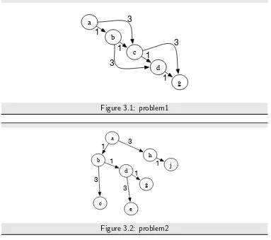
The first search problem is one with 5 nodes where the least-cost path is one

with many arcs. See Figure 3.1. Note that this example is used for the unit tests,

so the test (in

searchGeneric

) will need to be changed if this is changed.

150 problem1 = Search_problem_from_explicit_graph( 151 {'a','b','c','d','g'},

152 [Arc('a','b',1), Arc('a','c',3), Arc('b','d',3), Arc('b','c',1), 153 Arc('c','d',1), Arc('c','g',3), Arc('d','g',1)],

154 start = 'a', 155 goals = {'g'})

The second search problem is one with 8 nodes where many paths do not lead

to the goal. See Figure 3.2.

157 problem2 = Search_problem_from_explicit_graph( 158 {'a','b','c','d','e','g','h','j'},

(36)

3

1

a

b

d c

g

Figure 3.1: problem1

3 3

3

1

1 1

1 a

b

c

d

e g

h j

Figure 3.2: problem2

160 Arc('d','g',1), Arc('a','h',3), Arc('h','j',1)], 161 start = 'a',

162 goals = {'g'})

The third search problem is a disconnected graph (contains no arcs), where the

start node is a goal node. This is a boundary case to make sure that weird cases

work.

164 problem3 = Search_problem_from_explicit_graph( 165 {'a','b','c','d','e','g','h','j'},

166 [],

167 start = 'g', 168 goals = {'k','g'})

The

acyclic delivery problem

is the delivery problem described in Example

3.4 and shown in Figure 3.2 of the textbook.

170 acyclic_delivery_problem = Search_problem_from_explicit_graph(

(37)

3.1. Representing Search Problems

37

192 start = 'o103',

193 goals = {'r123'}, 194 hmap = {

211 'storage' : 12

212 }

213 )

The

cyclic delivery problem

is the delivery problem described in Example

3.8 and shown in Figure 3.6 of the textbook. This is the same as

acyclic delivery problem

,

but almost every arc also has its inverse.

215 cyclic_delivery_problem = Search_problem_from_explicit_graph(

216 {'mail','ts','o103','o109','o111','b1','b2','b3','b4','c1','c2','c3', 217 'o125','o123','o119','r123','storage'},

(38)

219 Arc('o103','ts',8), Arc('ts','o103',8), 220 Arc('o103','b3',4),

221 Arc('o103','o109',12), Arc('o109','o103',12), 222 Arc('o109','o119',16), Arc('o119','o109',16), 223 Arc('o109','o111',4), Arc('o111','o109',4), 224 Arc('b1','c2',3),

225 Arc('b1','b2',6), Arc('b2','b1',6), 226 Arc('b2','b4',3), Arc('b4','b2',3), 227 Arc('b3','b1',4), Arc('b1','b3',4), 228 Arc('b3','b4',7), Arc('b4','b3',7), 229 Arc('b4','o109',7),

230 Arc('c1','c3',8), Arc('c3','c1',8), 231 Arc('c2','c3',6), Arc('c3','c2',6), 232 Arc('c2','c1',4), Arc('c1','c2',4),

233 Arc('o123','o125',4), Arc('o125','o123',4), 234 Arc('o123','r123',4), Arc('r123','o123',4), 235 Arc('o119','o123',9), Arc('o123','o119',9),

236 Arc('o119','storage',7), Arc('storage','o119',7)], 237 start = 'o103',

238 goals = {'r123'}, 239 hmap = {

240 'mail' : 26,

241 'ts' : 23,

242 'o103' : 21,

243 'o109' : 24,

244 'o111' : 27,

245 'o119' : 11,

246 'o123' : 4,

247 'o125' : 6,

248 'r123' : 0,

249 'b1' : 13,

250 'b2' : 15,

251 'b3' : 17,

252 'b4' : 18,

253 'c1' : 6,

254 'c2' : 10,

255 'c3' : 12,

256 'storage' : 12

257 }

258 )

3.2 Generic Searcher and Variants

To

run

the

search

demos,

in

folder

“

aipython

_”,

_load

(39)

3.2. Generic Searcher and Variants

39

3.2.1 Searcher

A

Searcher

for a problem can be asked repeatedly for the next path. To solve a

problem, we can construct a

Searcher

object for the problem and then repeatedly

ask for the next path using

search

. If there are no more paths,

None

is returned.

searchGeneric.py — Generic Searcher, including depth-first and A*

11 from display import Displayable, visualize 12

13 class Searcher(Displayable):

14 """returns a searcher for a problem.

15 Paths can be found by repeatedly calling search(). 16 This does depth-first search unless overridden 17 """

18 def __init__(self, problem):

19 """creates a searcher from a problem 20 """

21 self.problem = problem 22 self.initialize_frontier() 23 self.num_expanded = 0

24 self.add_to_frontier(Path(problem.start_node())) 25 super().__init__()

26

27 def initialize_frontier(self): 28 self.frontier = []

29

30 def empty_frontier(self): 31 return self.frontier == [] 32

38 """returns (next) path from the problem's start node

39 to a goal node.

40 Returns None if no path exists. 41 """

42 while not self.empty_frontier(): 43 path = self.frontier.pop()

44 self.display(2, "Expanding:",path,"(cost:",path.cost,")")

45 self.num_expanded += 1

46 if self.problem.is_goal(path.end()): # solution found

47 self.display(1, self.num_expanded, "paths have been expanded and", 48 len(self.frontier), "paths remain in the frontier") 49 self.solution = path # store the solution found

50 return path

51 else:

(40)

55 self.add_to_frontier(Path(path,arc)) 56 self.display(3,"Frontier:",self.frontier) 57 self.display(1,"No (more) solutions. Total of", 58 self.num_expanded,"paths expanded.")

Note that this reverses the neigbours so that it implements depth-first search

in an intutive manner (expanding the first neighbor first). This might not be

required for other methods.

Exercise 3.1

When it returns a path, the algorithm can be used to find another path by calling search

()

again. However, it does not find other paths that go through one goal node to another. Explain why, and change the code so that it can find such paths whensearch

()

is called again.

3.2.2 Frontier as a Priority Queue

In many of the search algorithms, such as

A

∗

and other best-first searchers, the

frontier is implemented as a priority queue. Here we use the Python’s built-in

priority queue implementations,

heapq

_.

Following the lead of the Python documentation,

http://docs.python.org/

3.3/library/heapq.html

, a frontier is a list of triples. The first element of each

triple is the value to be minimized. The second element is a unique index which

specifies the order when the first elements are the same, and the third element

is the path that is on the queue. The use of the unique index ensures that the

priority queue implementation does not compare paths; whether one path is

less than another is not defined. It also lets us control what sort of search (e.g.,

depth-first or breadth-first) occurs when the value to be minimized does not

give a unique next path.

The variable

frontier index

is the total number of elements of the frontier

that have been created. As well as being used as a unique index, it is useful for

statistics, particularly in conjunction with the current size of the frontier.

searchGeneric.py — (continued)

60 import heapq # part of the Python standard library 61 from searchProblem import Path

62

63 class FrontierPQ(object):

64 """A frontier consists of a priority queue (heap), frontierpq, of 65 (value, index, path) triples, where

66 * value is the value we want to minimize (e.g., path cost + h). 67 * index is a unique index for each element

68 * path is the path on the queue

69 Note that the priority queue always returns the smallest element. 70 """

71

72 def __init__(self):

73 """constructs the frontier, initially an empty priority queue 74 """

1 Python code for Artificial Intelligence: Foundations of Computational Agents

1

Python code for Artificial

Intelligence: Foundations of

Computational Agents

David L. Poole and Alan K. Mackworth

Version 0.7.6 of August 20, 2018.

http://aipython.org

http://artint.info

©David L Poole and Alan K Mackworth 2017.

All code is licensed under a Creative Commons

Attribution-NonCommercial-ShareAlike 4.0 International License. See:

http://creativecommons.org/licenses/

by-nc-sa/4.0/deed.en US

This document and all the code can be downloaded from

http://artint.info/AIPython/

or from

http://aipython.org

Contents

Contents

3

1

Python for Artificial Intelligence

7

1.1

Why Python? . . . .

7

1.2

Getting Python . . . .

7

1.3

Running Python . . . .

8

1.4

Pitfalls . . . .

9

1.5

Features of Python . . . .

9

1.6

Useful Libraries . . . .

13

1.7

Utilities . . . .

14

1.8

Testing Code . . . .

17

2

Agents and Control

19

2.1

Representing Agents and Environments . . . .

19

2.2

Paper buying agent and environment . . . .

20

2.3

Hierarchical Controller . . . .

23

3

Searching for Solutions

31

3.1

Representing Search Problems . . . .

31

3.2

Generic Searcher and Variants . . . .

38

3.3

Branch-and-bound Search . . . .

44

4

Reasoning with Constraints

49

4.1

Constraint Satisfaction Problems . . . .

49

4.2

Solving a CSP using Search . . . .

_{or from}