DAILY ESTIMATION OF FINE PARTICULATE MATTER MASS CONCENTRATION
THROUGH SATELLITE BASED AEROSOL OPTICAL DEPTH
H.Karimiana,b*, Q.Lia,b*, C.C.Lic, J.Fana,b, L,Jina,b, C.Gonga,b, Y.Moa,b, J,Houa,b, A,Ahmadd
a
School of Earth and Space Science, Peking University, Beijing 100871, China-(hamedk,liqi)@pku.edu.cn b
Beijing Advanced Innovation Center for Future Internet Technology, Beijing, China c
Department of Atmospheric and Oceanic Sciences, School of Physics, Peking University, Beijing, 100871, China d
Institute of Geospatial Science and Technology, University Technology Malaysia,Skudai,81310,Malaysia
KEY WORDS: Geographically Weighted Regression, Statistical Model, PM2.5, MODIS, Aerosol Optical Depth
ABSTRACT:
Estimating exposure to fine Particulate Matter (PM2.5)requires surface with high spatial resolution. Aerosol optical depth (AOD) is one of MODIS products, being used to monitor PM2.5 concentration on ground level indirectly. In this research, AOD was derived in fine spatial resolution of 1×1 Km by utilizing an algorithm developed in which local aerosol models and conditions were took into account. Afterwards, due to spatial varying the relation between AOD-PM2.5, a regional scale geographically weighted regression model (GWR) was developed to derive daily seamless surface concentration of PM2.5 over Beijing, Tianjin and Hebei. For this purpose , various combinations of explanatory variables were investigated in the base of data availability, among which the best one includes AOD, PBL height, mean value of RH in boundary layer, mean value of temperature in boundary layer, wind speed and pressure was selected for the proposed GWR model over study area. The results show that, our model produces surface concentration of PM2.5 with annual RMSE of 18.6μg/m
3
. Besides, the feasibility of our model in estimating air pollution level was also assessed and high compatibility between model and ground monitoring was observed, which demonstrates the capability of the MODIS AOD and proposed model to estimate ground level PM2.5.
1. INTRODUCTION
Aerosols or particulate matters can be defined as a system of solids or liquids suspended in gaseous environments such as air in radios varies from some nanometre to larger than 100 micrometre. The major concentration of the atmospheric aerosols is found in troposphere and its bottom layer which is called Planetary Boundary Layer (PBL), as most production sources of aerosols are located in this layer (Kulkarni et al., 2010).One of the major negative aspects of aerosols is their adverse effects on human health. In general, the finer the size of the particulate matter is, the deeper it can penetrate inside the respiration system where the absorption is more serious. There are a pile of papers investigating the adverse effects of particulate matters on health from them it can be concluded that measurement of ground level fine particulate matters (PM2.5,particles with diameters less than 2.5 μm) is the fundament for epidemiological studies and sustainable development (Fuzzi et al., 2015; Karimian et al., 2012; Pope and Dockery, 2006).In spite of efforts done by China to control air pollutants emissions, there are reports of increasingly occurrence of haze or smog episodes followed by the high PM2.5 level and diminished visibility especially in mega cities of China (Kan et al., 2009; Zhang and Cao, 2015). China has started to disclose hourly pollutant concentrations to the public since January 2013. One of the major short comings of ground level monitoring stations is their coarse spatial coverage, especially those are used in epidemiological studies where the finer special coverage is required.
One of remote sensing products is atmospheric Aerosol Optical Depth (AOD) that can be defined as the degree to which aerosols prevent the transmission of light by absorption or scattering. The capability of AOD in monitoring PM2.5 has been demonstrated in a number of studies (Chu et al., 2016). MODerate resolution Image
Due to heterogeneous nature of the AOD and PM2.5, monitoring of PM2.5 through AOD is a challenging task. Since from on hand, AOD is unit less sunlight attenuation due to the existence of atmospheric aerosols in the vertical column (ground to top of the atmosphere), while PM2.5 is dry mass of fine particles measure in ground surface. Previous studies which retrieve PM2.5 from satellite based AOD started with two variable empirical regression models proposed in different regions(Hoff and Christopher, 2009). As the consequence of the disagreement between correlation coefficients in different regions, it was concluded that beside AOD, other factors also have influences in this correlation, such as humidity, wind direction and speed, land use, aerosols type and height of boundary layer (Chu et al., 2016). Hence as an approach, global and regional chemical transport models (CTM) were exploited to estimate PM2.5 through simulating the effective factors (Emmons et al., 2010; Liu, 2004; Pfister et al., 2011; van Donkelaar et al., 2006; van Donkelaar et al., 2013). Although CTMs provide spatially continues information about air pollutants without requiring ground PM2.5 and their performance will be improved by assimilation of satellite based AOD (Chen et al., 2014), their spatial resolution is coarse yet for epidemiological studies. Moreover, due to the lack of pollutants emissions type and emissions listing data in developing countries, it is hard to meet the conditions that required to apply in CTMs, resulting the numerical model uncertainties (Chu et al., 2016). Another widely used approach is observation based methods which relies on application of statistical techniques to estimate PM2.5 as the dependant variable, through combining AOD with several covariates as predictors. Among these aforementioned methods, Semi empirical linear regression models have been proposed based on physical understanding of the correlation between AOD and PM2.5 by including boundary layer height and hygroscopic growth factors (Chu et al., 2013; Li et al., 2005b). Karimian et al. (2016) claimed that incorporating the vertical profile of relative humidity instead of ground level solely and aerosol size distribution could improve the AOD-PM2.5 correlation. To improve the accuracy of the estimated PM2.5 more complex statistical models and machine learning methods such as mixed effect model, general additives model, land use regression, Bayesian hierarchical model, back propagation neural network and artificial neural network have been developed using different sets of covariates (Chu et al., 2016; Liu et al., 2009; Ma et al., 2014; Wu et al., 2012; Xie et al., 2015; Zhan et al., 2017). Due to the variety of sources that produce fine particulate matters, concentration and chemical composition of PM2.5 can vary in short distance(Kumar, 2010). Consequently, optical properties of the particles which influenced by chemical composition vary as well. Therefore, considering this variety in aerosol type is necessary in linkage between AOD-PM2.5. The effect of the aerosol type variation in the statistical model can be take in to account if a local scale model could be utilized instead of global scale model. In the oppose to global regression models which give one value for the entire study area, Geographically Weighted Regression (GWR) (a local regression method), considers the non stationary and spatial heterogeneity of the relation between explained and explanatory variables(Fotheringham et al., 2002 ). As the result, in this study we proposed a GWR based model to produce seamless surface of PM2.5 using AOD 1km in Beijing, Tianjin and Hebei (BTH) area for whole year 2013.
Figure 1.Spatial distribution of ground monitoring PM2.5 stations (green pin for model calibration, blue
pin for validation of the model)
2. STUDY AREA AND DATA
2.1 Study Area
The study area, including Beijing, Tianjin and Hebei (~ 113⁰ -120⁰ E, 36⁰-43⁰ N) is one of regions suffering from frequent and sever air pollution scenarios. Beijing, the capital city is located in this area with high population density. This area is in a warm temperate zone with typical continental monsoon climate(Chen, 2014). It is placed at the northern tip of north China plain being open to the south and east and surrounded by mountains in north, northwest and west, that may make the formation of the haze easier , by considering air pollution emission sources located in south and east (He et al., 2012; Li and Shao, 2009).
2.2 Satellite Data
Finer resolution of satellite AOD can improve the PM2.5 derived from satellite data. Therefore, AOD with fine spatial resolution of (1km×1km) was retrieved for the whole year of 2013 over the study area, which makes our study differ from studies using 10 km or 3 km AOD data. As the AOD is reported in visible range, only daytime MODIS data (~10:30 Terra, ~13:30 Aqua; local time) was processed following the algorithm developed by Li et al. (2005a). The Estimated retrieval errors are within 15% to 20% by validation compared with sun-photometer measurements, which is of the same accuracy as MODIS standard aerosol products over Beijing and Hong Kong (Li et al., 2005a; Lin et al., 2015). The retrieved AOD (Y) was validated by the comparison to AERONET level 1.5 AOD (X), which was observed at the7 AERONET stations located in eastern part of China. It exhibited a correlation coefficient of R= 0.79, with a slope of 0.73 and intercept of 0.12, and suggested that MODIS AOD correlated well with sun-photometer observations (Lin et al., 2015).
2.3 Ground Level PM2.5
This study used hourly PM2.5 concentration data for entire 2013. According to the Chinese National Ambient Air Quality Standard (CNAAQS, GB3095-2012, available on the Chinese Ministry of Environmental Protection (MEP) Web
Tianjin Hebei
site http://kjs.mep.gov.cn/)(Ma et al., 2014), the ground PM2.5 data of China’s mainland are measured with the tapered element oscillating microbalance (TEOM) technique or beta attenuation monitors (BAM or β-gauge). Data are recorded on hourly base, and meet the control limit of 10% for both accuracy and precision (EPD, 2013). There are 79 stations located within the study area, among which 60 stations were used for model calibration with the remaining 19 stations were used for model validation .The data close to MODIS overpass time was collected for further processing(Figure 1).
2.4 Model Based Meteorology Data
Global Forecast System (GFS) is a numeric weather prediction under the authority of national centre of environment prediction. The numerical models (atmosphere, ocean, land, and sea ice) are run together four times daily and produce global covered forecast for up to 16 days. The globally covered data was obtained from the GFS official website in the horizontal resolution of 0.5⁰ at the MODIS over pass time initially. Afterwards, the data over study area extracted in the 0.5 ⁰×0.5⁰ grids through self programming. Each GFS file includs several data covering geo-potential height in different pressure level, boundary layer height, relative humidity (8 levels), temperature (8 levels) and wind north(v) and east(u) components from that, wind speed(Ws) GWR, a weight is ascribed to each observation, based on the distance of the data point from the regression point (distance decay based weight) using a continuous weighting function such as Gaussian or bi-square (spatial kernel function). Taking the weight into consideration, data closer to regression point get higher weight than the further one. In accordance to the fact that, GWR is sensitive to multicolinearity (redundancy) of the explanatory variables, which in simple words means two or more variables say the same story and play the same role in model. Hence in the first step we checked the redundancy of the explanatory variables by applying a linear regression between each two auxiliary variables (Table 1). As can be seen, except the correlation between topography (Topo) and pressure (Press) that express redundancy (R=0.99), the rest of variables exhibit no redundancy. Therefore, we eliminated the model which includes both Topo and Press value together. In the second stage, because the meteorological data (including wind, surface pressure, surface temperature, averaged surface in boundary layer, RH in the surface, averaged RH in the boundary layer and PBL height) is reported in course spatial resolution(0.5○×0.5○) we assimilated all data to the pixel with special resolution of 5 Km using Kriging method. Next, the meteorology and AOD values over each ground PM2.5 station were extracted. With all required data collected, we used GWR4 to perform GWR model over study area and extract the surface PM2.5 concentration. One remarkable aspect of GWR is the capability in the case where not well distributed data points exist (spares data around regression point)(Ma et al., 2014). Due to the reason mentioned before, there are two type of method used for selecting bandwidth which are known as fixed (which is set fixed for all regression point) or
adaptive (kernel has a larger bandwidth when points are spares, and narrower when points are plenty).Adaptive bandwidth is the optimal bandwidth selected so that there are the same number of data points for each regression point. There are several strategies in determining optimal adaptive bandwidth (Guo et al., 2008). Akaike Information Criterion (AICc) was used to determine the optimal bandwidth , and details can be found in Fotheringham et al. (2002 ). As GWR could be used to determine the best model among different models with various explanatory variables with the usage of AICc, we tried different combinations (8) to get the best one (the lowest value of AICc assigned to the best model). Table 2 provides the monthly averaged performance of different combinations.
Table1. Correlation between explanatory variables used in GWR model
Since one of the objectives of this study was testing the role of vertical profile of RH and temperature in model’s performance, mean values of these two parameters inside PBL were calculated and compared with the performance of the models calibrated with ground level value solely. In the table RH_surface(%) indicate the relative humidity value in ground level , RH_m (%) stands for the mean value in boundary layer, T_sur (⁰C)and T_m(⁰C) indicates surface value and mean value of temperature in boundary layer respectively. Wind is the speed of wind (m/s) measured at 10 meter above the ground derived from (u,v) data. Topo stands for topography, Press for surface level pressure (hpa) and of temperature and relative humidity in boundary layer.
Table2. Assessing of different model combination regarding to AICc and R2
Combination AICc R2
AOD-PM 552.5 0.4
AOD-PM-PBL-RHsur 542 0.56
AOD-PM-PBL-RHm 539.2 0.61
AOD-PM-PBL-RHsur-Tsur 534.1 0.62
AOD-PM-PBL-RHm-Tm 531.8 0.64
AOD-PM-PBL-RHm-Tm-Wind 527.4 0.69
AOD-PM-PBL-RHm-Tm-Wind-Topo 524 0.73
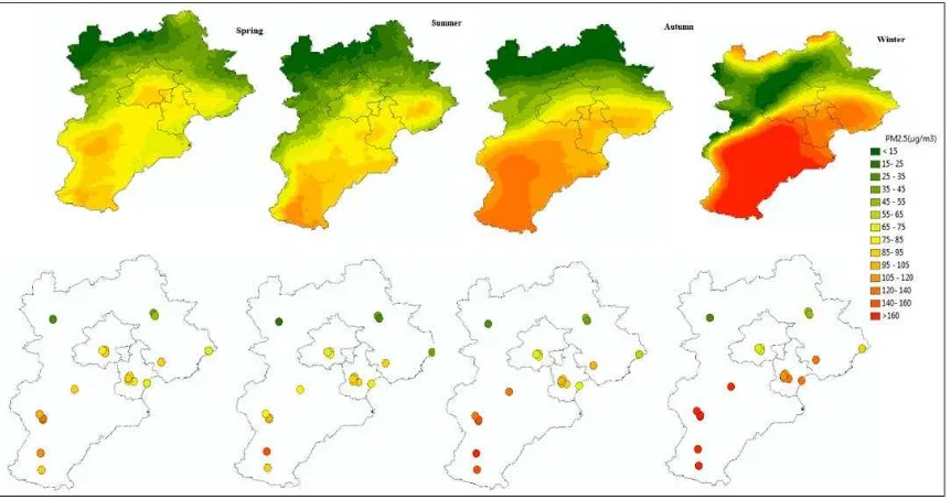
Figure2. Spatial and temporal (seasonal) variation of PM2.5 derived from GWR (upper) and comparison with ground observation (lower)
Considering meteorological parameters can improve the performance of the model remarkably (from 552 to 523), and better performance is observed when the vertical profile of RH and T, other than ground level, where taken into account. The gained correlation is compatible with the study done over south of China, where the authors cited their GWR model got correlation coefficient of 0.74 (Song et al., 2014). Consequently we applied the best combination as our GWR model over BTH. The unites of parameters involve in model were explained above.
PM2.5~AOD+PBL+RHm+Tm+Ws+Press (2)
In order to get surface distribution of PM2.5 we applied the spatial varied regression coefficients derived from GWR model from each pixel through multiplying to model parameters and add diagonal elements of this matrix to the model Intercept to get the PM2.5 concentration for each pixel.
4. RESULTS and DISCUSSION
4.1 Spatially Varying the Correlation
Figure (2) exhibits the spatial and seasonal variation of PM2.5 concentration derived from GWR model in 5 Km spatial resolution. In order to validate our model, we use 19 ground level PM2.5 monitoring stations as control data source (Figure 1). One of main advantages of using satellite data in particulate matter monitoring is providing the surface distribution in oppose to ground level observations, which have limited spatial coverage. As can be seen from the figure, southern part of the study area (Hebei) faces higher concentration of the fine particulate matter than other areas. This may be caused by the higher concentration of industrial and anthropogenic activities in that area. In the oppose of southern part, northern part which is a mountainous area with lower population density, exhibits considerably lower concentration. This proves the importance of anthropogenic activities as one of main sources that could generate PM2.5. Moreover, we can see a higher concentrations (above 160 μg/m3
) that is near 5 times more than the China
Figure 3.The spatial distribution of the annual PM2.5 concentration from developed GWR model (left) and comparison with ground observation (RMSE=18.6μg/m3
)
standard concentration (35μg/m3) in cold seasons (winter and autumn). This verifies the role that heating system plays in pollution by utilizing coal in study area. As can be seen there is a very good agreement between model performance and ground observations which determine the ability of our developed GWR model for PM2.5 estimation. The mean annual concentration of PM2.5 derived from GWR is shown in figure (3). As it is illustrated, most of study area face with moderate to unhealthy level of PM2.5 concentration, except northern regions. Compared with ground control observations (19 stations) the annual mean RMSE gains 18.6μg/m3
. This distribution pattern follows the distribution of PM2.5 derived from GWR for entire china with RMSE 30μg/m3
and 50 Km spatial resolution (Ma et al., 2014). Our model also exhibits better performance than a linear mixed effect model developed over BTH for 2013 with RMSE 23.1μg/m3 (Zheng et al., 2016). Also this result is compatible with the mixed effect model developed by Xie et al. (2015) over Beijing with annual RMSE 18((μg/m3
). This slightly better result may due to the more ground stations (well distributed N=35) that were used to calibrate the model.
Therefore, applying MODIS AOD and good combination of auxiliary data is recommended in future studies in the region suffering from lack of ground level fine particulate matter monitoring .GWR model is based on this concept that residuals have no spatial clustering and distribute randomly. Therefore, a good model is the one of which residuals are not clustered. As the result, we run Moran’s I model to check for spatial autocorrelation on residuals. The Moran’s I value, ranging from -1 (dispersion) to +1 (absolute autocorrelation) , 0 is the indicator of random distribution(Wang et al., 2005). In our study residuals distribute randomly and our model is acceptable from this aspect (Moran’s I index= 0.1).
4.2Applicability to Air Quality Monitoring
The major goal of monitoring air pollutants in urban areas is to improve air quality and health. The Air Quality Index (AQI) and air pollution level is designed based on six major atmospheric air pollutants concentration (SO2, NO2, CO, O3, PM10, and PM2.5). The AQI is calculated based on each pollutant concentration separately and reported corresponding to the highest AQI. Considering the fact that PM2.5 is one of the major pollutants in study area and most AQI is reported in accordance with PM2.5 concentration (Karimian et al., 2016) , we validate our model capability to monitor air pollution level .Table (3) illustrates the air quality and air pollution sub-index level based on corresponding PM2.5 concentrations (Zheng et al., 2014).
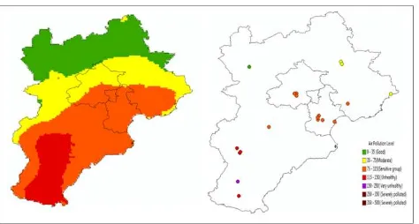
Figure 4 illustrates the air pollution level derived based on mean annual concentration of PM2.5 from GWR and the comparison with the one derived from observation based data. As can be seen, unhealthy level of air pollution was observed in large portion of the study area in 2013 and people living in BTH were exposed to long term level of unhealthy concentration of PM2.5. Moreover, as it is illustrated except for one station (located in southern part of the study area), satellite derived PM2.5 has this ability to estimate true air pollution level in study area. These results verify the ability of MODIS aerosol optical depth to be utilized in fine particulate matter studies. It is emphasized that, inclusion of meteorological parameters such as wind speed, pressure, temperature and especially boundary layer height and relative humidity (vertical profile) can improve the model performance. However, extension of the study area and well distribution of the data used to calibrate the model have influence on performance of the model.
Table3. AQI and air pollution levels with corresponding PM2.5 concentrations (Ministry of Environmental Protection
of People’s Republic of China)
5.CONCLUSIONS
In spite of accuracy and high temporal resolution, ground level monitoring of PM2.5 is suffering from course spatial
Figure4. The annual spatial distribution of the air pollution level based on PM2.5 concentration from the GWR (left)
and comparison with air pollution level from ground observation(right)
resolution especially for epidemiological purposes. In this study a regional scale geographically weighted regression model was developed in order to retrieve daily seamless surface concentration of PM2.5 over Beijing, Tianjin, Heibei using satellite based AOD with 1×1 Km spatial resolution. Because the main source of fine particulate matter is from anthropogenic activities, their type and chemical composition varies in large area. The spatial variability and non stationary of the relation can be considered in GWR as a local statistic model. Several models with various combinations of explanatory variables were investigated and the best combination including AOD, PBL height, and mean value of RH in boundary layer, mean value of temperature in boundary layer, wind speed and pressure was selected as the explanatory variable of the proposed GWR model over study area.
The feasibility of the proposed model was examined using 19 control stations distributed over BTH with the annual mean RMSE= 18.6 μg/m3. Besides, it was shown that our model has this ability to monitor air pollution level and the results are highly compatible with ground monitoring ones. However, some of the issues should be carried in mind before using GWR model. First comes to the study area where should be large enough to detect the correlation variation by the model. Second issue is data should be distributed well in study area. In future studies models to compensate for missing AOD data (non retrieved days) should be proposed. Moreover, capability of different statistical models in estimation of PM2.5 through AOD can be investigated and compared.
ACKNOWLEDGMENTS
The study was supported by the National Key Technology R&D Program of Ministry of Science and Technology of China (Grant Number: 2012BAC20B06).
REFERENCES
Chen, D., Liu, Z., Schwartz, C.S., Lin, H.C., Cetola, J.D., Gu, Y., Xue, L., 2014. The impact of aerosol optical depth assimilation on aerosol forecasts and radiative effects during a wild fire event over the United States. Geoscientific Model Development 7,pp. 2709-2715.
AQI Air pollution level Max PM2.5 (μg/m3)
50 Good 35
100 Moderate 75
150 Sensitive Group 115
200 Unhealthy 150
Chen, J., 2014. Impact of Relative Humidity and Water Soluble Constituents of PM2.5 on Visibility Impairment in Beijing, China. Aerosol and Air Quality Research 14,pp.260-268. Concentration Using Satellite Aerosol Optical Depth. Atmosphere 7, 129. Related chemical Tracers, version 4 (MOZART-4). Geoscientific Model Development 3,pp. 43–67.
Fotheringham, S.A., Brunsdon, C., Charlton, M., 2002 Geographically Weighted Regression the analysis of spatially varying relationships. Wiley, England.
Fuzzi, S., Baltensperger, U., Carslaw, K., Decesari, S., Denier van der Gon, H., 2015. Particulate matter, air quality and climate: lessons learned and future needs. Atmospheric Chemistry and Physics 15,pp. 8217-8299.
Guo, L., Ma, Z., Zhang, L., 2008. Comparison of bandwidth selection in application of geographically weighted regression: a case study. Canadian Journal of Forest Research 38, pp. 2526-2534.
He, Q., Li, C., Geng, F., Lei, Y., Li, Y., 2012. Study on Long-term Aerosol Distribution over the Land of East China Using MODIS Data. Aerosol and Air Quality Research 12, pp.304-319.
Hoff, M.R., Christopher, A.S., 2009. Remote Sensing of Particulate Pollution from Space: Have We Reached the Promised Land? Journal of the Air & Waste Management Association 59, pp. 645–675.
Kan, H., Chen, B., Hong, C., 2009. Health impact of outdoor air pollution in China: current knowledge and future research needs. Environ Health Perspect 117, 187.
Karimian, H., Li, Q., Chen, H.F., 2012. Assessing Urban Sustainable Development in Isfahan. Applied Mechanics and Materials 253-255, pp. 244-248.
Karimian, H., Li, Q., Li, C., Jin, L., Fan, J., Li, Y., 2016. An Improved Method for Monitoring Fine Particulate Matter Mass Concentrations via Satellite Remote Sensing. Aerosol and Air Quality Research 16, pp. 1081-1092.
Kaufman, Y.J., Tanre, D., Boucher, O., 2002. A satellite view of aerosols in the climate system Nature 419, pp. 215–223.
King, M., Menzel, W.P., Kaufman, Y.J., Tanre, D., Gao, B., 2003. Cloud and aerosol properties, precipitable water, and profiles of temperature and water vapor from MODIS. IEEE
Transactions on Geoscience and Remote Sensing 41,pp.442– 458.
Kulkarni, P., Baron, P., Willeke, K., 2010. Aerosol Measurement:Principle,Techniques and Applications, 3rd ed. Willey & Sons.
Kumar, N., 2010. What Can Affect AOD–PM2.5 Association? Environ.Health Persp. 118 |, 109.
Levy, R.C., Mattoo, S., Munchak, L.A., Remer, L.A., Sayer, A.M., Hsu, N.C., 2013. The Collection 6 MODIS aerosol X.Y., 2005b. Application of MODIS satellite products to the air pollution research in Beijing. Sci. China Ser.D 48, pp.209-219. high-resolution distribution of ground-level PM2.5. Remote Sens.Environ. 156,pp.117-128.
Liu, Y., 2004. Mapping annual mean ground-level PM2.5concentrations using Multiangle Imaging Spectroradiometer aerosol optical thickness over the contiguous United States. J.Geophys.Res. 109.
Liu, Y., Paciorek, C.J., Koutrakis, P., 2009. Estimating regional spatial and temporal variability of PM(2.5) concentrations using satellite data, meteorology, and land use information. Environmental health perspectives 117, pp. 886-892.
Lyapustin, A., Wang, Y., Laszlo, I., Kahn, R., Korkin, S., Remer, L., Levy, R., Reid, J.S., 2011. Multiangle implementation of atmospheric correction (MAIAC): 2. Aerosol algorithm. J.Geophys.Res. 116.
Pope, A.C., Dockery, D., 2006. Health Effects of Fine Particulate Air Pollution: Lines that Connect. J.Air Waste Manage.Assoc. 56,pp. 709-742.
Song, W., Jia, H., Huang, J., Zhang, Y., 2014. A satellite-based geographically weighted regression model for regional PM2.5 estimation over the Pearl River Delta region in China. Remote Sens. Environ, pp. 154, 1-7.
van Donkelaar, A., Martin, R.V., Park, R.J., 2006. Estimating ground-level PM2.5using aerosol optical depth determined from satellite remote sensing. J.geophys.Res. 111.
van Donkelaar, A., Martin, R.V., Spurr, R.J.D., Drury, E., Remer, L.A., Levy, R.C., Wang, J., 2013. Optimal estimation for global ground-level fine particulate matter concentrations. J.Geophys.Res.Atmos. 118, pp. 5621-5636.
Wang, Q., Ni, J., Tenhunen, J., 2005. Application of a geographically‐weighted regression analysis to estimate net primary production of Chinese forest ecosystems. Global Ecology and Biogeography 14, pp.379-393.
Wu, Y., Guo, J., Zhang, X., Tian, X., Zhang, J., Wang, Y., Duan, J., Li, X., 2012. Synergy of satellite and ground based observations in estimation of particulate matter in eastern China. The Science of the total environment 433,pp. 20-30.
Xie, Y., Wang, Y., Zhang, K., Dong, W., Lv, B., Bai, Y., 2015. Daily Estimation of Ground-Level PM2.5 Concentrations over Beijing Using 3 km Resolution MODIS AOD. Environmental science & technology 49,pp. 12280-12288.
Zhan, Y., Luo, Y., Deng, X., Chen, H., Grieneisen, M.L., Shen, X., Zhu, L., Zhang, M., 2017. Spatiotemporal prediction of continuous daily PM 2.5 concentrations across China using a spatially explicit machine learning algorithm. Atmospheric Environment 155,pp. 129-139.
Zhang, Y.L., Cao, F., 2015. Fine particulate matter (PM 2.5) in China at a city level. Sci Rep 5, 14884.
Zheng, S., Cao, C.X., Singh, R.P., 2014. Comparison of ground based indices (API and AQI) with satellite based aerosol products. Sci.Total Environ. 488-489,pp. 398-412.