arXiv:1711.06656v1 [math.OC] 17 Nov 2017
A Parallelizable Acceleration Framework for Packing Linear Programs
Palma London
California Institute of TechnologyShai Vardi
California Institute of Technology [email protected]
Adam Wierman
California Institute of TechnologyHanling Yi
The Chinese University of Hong Kong [email protected]
Abstract
This paper presents an acceleration framework for packing linear programming problems where the amount of data avail-able is limited, i.e., where the number of constraintsm is
small compared to the variable dimensionn. The framework
can be used as a black box to speed up linear programming solvers dramatically, by two orders of magnitude in our ex-periments. We present worst-case guarantees on the quality of the solution and the speedup provided by the algorithm, showing that the framework provides an approximately op-timal solution while running the original solver on a much smaller problem. The framework can be used to accelerate exact solvers, approximate solvers, and parallel/distributed solvers. Further, it can be used for both linear programs and integer linear programs.
1
Introduction
This paper proposes a black-box framework that can be used to accelerate both exact and approximate linear program-ming (LP) solvers for packing problems while maintaining high quality solutions.
LP solvers are at the core of many learning and inference problems, and often the linear programs of interest fall into the category ofpacking problems. Packing problems are lin-ear programs of the following form:
maximize Pn
j=1cjxj (1a)
subject to Pn
j=1aijxj ≤bi i∈[m] (1b)
0≤xj≤1 j∈[n] (1c)
whereA∈[0,1]m×n,b∈Rm
≥0,c∈Rn≥0.
Packing problems arise in a wide variety of set-tings, including max cut (Trevisan 1998), zero-sum matrix games (Nesterov 2005), scheduling and graph embedding (Plotkin, Shmoys, and Tardos 1995), flow controls (Bartal, Byers, and Raz 2004), auction mecha-nisms (Zurel and Nisan 2001), wireless sensor networks
Copyright c2018, Association for the Advancement of Artificial Intelligence (www.aaai.org). All rights reserved.
Funding: PL, SV, and AW were supported in part by NSF grants AitF-1637598, CNS-1518941, CPS-154471 and the Linde Insti-tute. HY was supported by the International Teochew Doctors As-sociation Zheng Hanming Visiting Scholar Award Scheme.
(Byers and Nasser 2000), and many other areas. In ma-chine learning specifically, they show up in an array of problems, e.g., in applications of graphical models (Ravikumar, Agarwal, and Wainwright 2010), associative Markov networks (Taskar, Chatalbashev, and Koller 2004), and in relaxations of maximum a posteriori (MAP) esti-mation problems (Sanghavi, Malioutov, and Willsky 2008), among others.
In all these settings, practical applications require LP solvers to work at extreme scales and, despite decades of work, commercial solvers such as Cplex and Gurobi do not scale as desired in many cases. Thus, despite a large litera-ture, the development of fast, parallelizable solvers for pack-ing LPs is still an active direction.
Our focus in this paper is on a specific class of packing LPs for which data is either very costly, or hard to obtain. In these situationsm ≪ n; i.e., the number of data points mavailable is much smaller than the number of variables, n. Such instances are common in areas such as genetics, astronomy, and chemistry. There has been considerable research focusing on this class of problems in recent years, in the context of LPs (Donoho and Tanner 2005; Bienstock and Iyengar 2006) and also more gener-ally in convex optimization and compressed sensing (Candes, Romberg, and Tao 2006; Donoho 2006), low rank matrix recovery (Recht, Fazel, and Parrilo 2010; Candes and Plan 2011), and graphical models (Yuan and Lin 2007a; Mohan et al. 2014).
Contributions of this paper. We present a black-box ac-celeration framework for LP solvers. When given a packing LP and an algorithmA, the framework works by sampling anǫs-fraction of the variables and usingAto solve LP (1)
restricted to these variables. Then, the dual solution to this sampled LP is used to define a thresholding rule for the pri-mal variables of the original LP; the variables are set to ei-ther 0 or1 according to this rule. The framework has the following key properties:
1. It can be used to accelerate exact or approximate LP-solvers (subject to some mild assumptions which we dis-cuss below).
2. Since the original algorithmA is run only on a (much smaller) LP withǫs-fraction of the variables, the
3. The threshold rule can be used to set the values of the vari-ables in parallel. Therefore, ifAis a parallel algorithm, the framework gives a faster parallel algorithm with neg-ligible overhead.
4. Since the threshold rule sets the variables to integral val-ues, the framework can be applied without modification to solve integer programs that have the same structure as LP (1), but with integer constraints replacing (1c).
There are two fundamental tradeoffs in the framework. The first is captured by the sample size,ǫs. Settingǫsto be
small yields a dramatic speedup of the algorithmA; how-ever, if ǫs is set too small the quality of the solution
suf-fers. A second tradeoff involves feasibility. In order to en-sure that the output of the framework is feasible w.h.p. (and not just that each constraint is satisfied in expectation), the constraints of the sample LP are scaled down by a factor de-noted byǫf. Feasibility is guaranteed ifǫf is large enough;
however, if it is too large, the quality of the solution (as mea-sured by the approximation ratio) suffers.
Our main technical result is a worst-case characterization of the impact ofǫsandǫf on the speedup provided by the
framework and the quality of the solution. Assuming that al-gorithmAgives a(1 +δ)approximation to the optimal so-lution of the dual, we prove that the acceleration framework guarantees a(1−ǫf)/(1 +δ)2-approximation to the optimal
solution of LP (1), under some assumptions about the input andǫf. We formally state the result as Theorem 3.1, and
note here that the result shows thatǫf grows proportionally
to1/√ǫs, which highlights that the framework maintains a
high-quality approximation even when sample size is small (and thus the speedup provided by the framework is large).
The technical requirements for ǫf in Theorem 3.1
im-pose some restrictions on both the family of LPs that can be provably solved using our framework and the algorithms that can be accelerated. In particular, Theorem 3.1 requires
minibi to be large and the algorithmAto satisfy
approx-imate complementary slackness conditions (see Section 2). While the condition on thebiis restrictive, the condition on
the algorithms is not – it is satisfied by most common LP solvers, e.g., exact solvers and many primal dual approxi-mation algorithms. Further, our experimental results demon-strate that these technical requirements are conservative – the framework produces solutions of comparable quality to the original LP-solver in settings that are far from satisfy-ing the theoretical requirements. In addition, the accelerator works in practice for algorithms that do not satisfy approxi-mate complementary slackness conditions, e.g., for gradient algorithms as in (Sridhar et al. 2013). In particular, our ex-perimental results show that the accelerator obtains solutions that are close in quality to those obtained by the algorithms being accelerated on the complete problem,andthat the so-lutions are obtained considerably faster (by up to two orders of magnitude). The results reported in this paper demon-strate this by accelerating the state-of-the-art commercial solver Gurobi on a wide array of randomly generated pack-ing LPs and obtainpack-ing solutions with<4%relative error and a more than 150×speedup. Other experiments with other solvers are qualitatively similar and are not included.
When applied to parallel algorithms, there are added op-portunities for the framework to reduce error while increas-ing the speedup, throughspeculative execution: the frame-work runs multiple clones of the algorithm speculatively. The original algorithm is executed on a separate sample and the thresholding rule is then applied by each clone in paral-lel, asynchronously. This improves both the solution quality and the speed. It improves the quality of the solution because the best solution across the multiple samples can be cho-sen. It improves the speed because it mitigates the impact of stragglers, tasks that take much longer than expected due to contention or other issues. Incorporating “cloning” into the acceleration framework triples the speedup obtained, while reducing the error by12%.
Summary of related literature. The approach un-derlying our framework is motivated by recent work that uses ideas from online algorithms to make of-fline algorithms more scalable, e.g., (Mansour et al. 2012; London et al. 2017). A specific inspiration for this work is (Agrawal, Wang, and Ye 2014), which introduces an online algorithm that uses a two step procedure: it solves an LP based on the first s stages and then uses the solution as the basis of a rounding scheme in later stages. The algo-rithm only works when the arrival order is random, which is analogous to sampling in the offline setting. However, (Agrawal, Wang, and Ye 2014) relies on exactly solving the LP given by the firstsstages; considering approximate so-lutions of the sampled problem (as we do) adds complexity to the algorithm and analysis. Additionally, we can leverage the offline setting to fine-tune ǫf in order to optimize our
solution while ensuring feasibility.
The sampling phase of our framework is reminiscent of the method of sketchingin which the data matrix is multi-plied by a random matrix in order to compress the problem and thus reduce computation time by working on a smaller formulation, e.g., see (Woodruff 2014). However, sketching is designed for overdetermined linear regression problems, m ≫n; thus compression is desirable. In our case, we are concerned with underdetermined problems,m ≪ n; thus compression is not appropriate. Rather, the goal of sampling the variables is to be able to approximately determine the thresholds in the second step of the framework. This differ-ence means the approaches are distinct.
The sampling phase of the framework is also reminiscent of the experiment designproblem, in which the goal is to solve the least squares problem using only a subset of avail-able data while minimizing the error covariance of the esti-mated parameters, see e.g., (Boyd and Vandenberghe 2004). Recent work (Riquelme, Johari, and Zhang 2017) applies these ideas to online algorithms, when collecting data for regression modeling. Like sketching, experiment design is applied in the overdetermined setting, whereas we consider the under-determined scenario. Additionally, instead of sam-pling constraints, we sample variables.
we use thresholding to “extend” the solution of a sam-pled LP to the full LP. The scheme we use is a deter-ministic threshold based on the complementary slackness condition. It is inspired by (Agrawal, Wang, and Ye 2014), but adapted to hold for approximate solvers rather than ex-act solvers. In this sense, the most related recent work is (Sridhar et al. 2013), which proposes a scheme for rounding an approximate LP solution. However, (Sridhar et al. 2013) uses all of the problem data during the approximation step, whereas we show that it is enough to use a (small) sample of the data.
A key feature of our framework is that it can be par-allelized easily when used to accelerate a distributed or parallel algorithm. There is a rich literature on distributed and parallel LP solvers, e.g., (Yarmish and Slyke 2009; Notarstefano and Bullo 2011; Burger et al. 2012; Richert and Cort´es 2015). More specifically, there is sig-nificant interest in distributed strategies for approximately solving covering and packing linear problems, such as the problems we consider here, e.g., (Luby and Nisan 1993; Young 2001; Bartal, Byers, and Raz 2004; Awerbuch and Khandekar 2008;
Allen-Zhu and Orecchia 2015).
2
A Black-Box Acceleration Framework
In this section we formally introduce our acceleration frame-work. At a high level, the framework accelerates an LP solver by running the solver in a black-box manner on a small sample of variables and then using a deterministic thresholding scheme to set the variables in the original LP. The framework can be used to accelerate any LP solver that satisfies the approximate complementary slackness condi-tions. The solution of an approximation algorithmAfor a family of linear programsFsatisfies the approximate com-plementary slackness if the following holds. Letx1, . . . , xn
be a feasible solution to the primal andy1, . . . , ymbe a
fea-sible solution to the dual.
• Primal Approximate Complementary Slackness: For αp ≥1andj ∈[n], ifxj >0thencj ≤Pmi=1aijyi ≤
αp·cj.
• Dual Approximate Complementary Slackness:Forαd ≥
1andi∈[m], ifyi>0thenbi/αd≤P n
i=1aijxj ≤bi.
We call an algorithmAwhose solution is guaranteed to sat-isfy the above conditions an(αp, αd)-approximation
algo-rithm forF. This terminology is non-standard, but is in-structive when describing our results. It stems from a foun-dational result which states that an algorithmAthat satisfies the above conditions is an α-approximation algorithm for any LP inFforα=αpαd (Buchbinder and Naor 2009).
The framework we present can be used to ac-celerate any (1, αd)-approximation algorithm.
While this is a stronger condition than simply re-quiring that A is an α-approximation algorithm, many common dual ascent algorithms satisfy this condition, e.g., (Agrawal, Klein, and Ravi 1995; Balakrishnan, Magnanti, and Wong 1989;
Bar-Yehuda and Even 1981; Erlenkotter 1978; Goemans and Williamson 1995). For example, the
Algorithm 1:Core acceleration algorithm
Input:Packing LPL, LP solverA,ǫs>0,ǫf >0
Output:xˆ∈Rn
1. Selects=⌈nǫs⌉primal variables uniformly at random.
Label this setS.
2. UseAto find an (approximate) dual solution
˜
y= [φ, ψ]∈[Rm,
Rs]to the sample LP. 3. Setxˆj =xj(φ)for allj∈[n].
4. Returnx.ˆ
vertex cover and Steiner tree approximation al-gorithms of (Agrawal, Klein, and Ravi 1995) and (Bar-Yehuda and Even 1981) respectively are both
(1,2)-approximation algorithms.
Given a(1, αd)-approximation algorithmA, the
acceler-ation framework works in two steps. The first step is to sam-ple a subset of the variables,S ⊂ [n],|S| = s = ⌈ǫsn⌉,
and useAto solve the followingsample LP, which we call LP (2). For clarity, we relabel the variables so that the sam-pled variables are labeled1, . . . , s.
maximize Ps
j=1cjxj (2a)
subject to Ps
j=1aijxj ≤(1
−ǫf)ǫs
αd bi i∈[m] (2b)
xj ∈[0,1] j∈[s] (2c)
Here, αd is the parameter of the dual approximate
com-plementary slackness guarantee ofA,ǫf > 0 is a
param-eter set to ensure feasibility during the thresholding step, andǫs > 0 is a parameter that determines the fraction of
the primal variables that are be sampled. Our analytic re-sults give insight for setting ǫf andǫs but, for now, both
should be thought of as close to zero. Similarly, while the results hold for anyαd, they are most interesting whenαd
is close to1(i.e.,αd = 1 +δfor smallδ). There are many
such algorithms, given the recent interest in designing ap-proximation algorithms for LPs, e.g., (Sridhar et al. 2013; Allen-Zhu and Orecchia 2015).
The second step in our acceleration framework uses the dual prices from the sample LP in order to set a threshold for a deterministic thresholding procedure, which is used to build the solution of LP (1). Specifically, letφ ∈ Rmand
ψ∈Rsdenote the dual variables corresponding to the con-straints (2b) and (2c) in the sample LP, respectively. We define the allocation (thresholding) rulexj(φ)as follows:
xj(φ) =
1 if Pm
i=1aijφi < cj
0 otherwise
We summarize the core algorithm of the acceleration framework described above in Algorithm 1. When imple-menting the acceleration framework it is desirable to search for the minimalǫfthat allows for feasibility. This additional
step is included in the full pseudocode of the acceleration framework given in Algorithm 2.
Algorithm 2:Pseudocode for the full framework. Input:Packing LPL, LP solverA,ǫs>0,ǫf >0
Output:xˆ∈Rn
Setǫf = 0.
whileǫf <1do
ˆ
x= Algorithm 1(L,A,ǫs,ǫf).
ifxˆis a feasible solution toLthen Returnx.ˆ
else
Increaseǫf.
a thresholding rule, the final solution output by the accelera-tor is integral. Thus, it can be viewed as an ILP solver based on relaxing the ILP to an LP, solving the LP, and round-ing the result. The difference is that it does not solve the full LP, but only a (much smaller) sample LP; so it pro-vides a significant speedup over traditional approaches. Sec-ond, the framework is easily parallelizable. The threshold-ing step can be done independently and asynchronously for each variable and, further, the framework can easily inte-grate speculative execution. Specifically, the framework can start multipleclones speculatively, i.e., take multiple sam-ples of variables, run the algorithmAon each sample, and then round each sample in parallel. This provides two bene-fits. First, it improves the quality of the solution because the output of the “clone” with the best solution can be chosen. Second, it improves the running time since it curbs the im-pact ofstragglers, tasks that take much longer than expected due to contention or other issues. Stragglers are a signifi-cant source of slowdown in clusters, e.g., nearly one-fifth of all tasks can be categorized as stragglers in Facebook’s Hadoop cluster (Ananthanarayanan et al. 2013). There has been considerable work designing systems that reduce the impact of stragglers, and these primarily rely on speculative execution, i.e., running multiple clones of tasks and choos-ing the first to complete (Ananthanarayanan et al. 2010; Ananthanarayanan et al. 2014; Ren et al. 2015). Running multiple clones in our acceleration framework has the same benefit. To achieve both the improvement in solution quality and running time, the framework runsK clones in parallel and chooses the best solution of the firstk < Kto complete. We illustrate the benefit of this approach in our experimental results in Section 3.
3
Results
In this section we present our main technical result, a worst-case characterization of the quality of the solution pro-vided by our acceleration framework. We then illustrate the speedup provided by the framework through experiments us-ing Gurobi, a state-of-the-art commercial solver.
3.1
A Worst-case Performance Bound
The following theorem bounds the quality of the solution provided by the acceleration framework. LetLbe a packing
LP withnvariables andmconstraints, as in (1), andB := mini∈[m]{bi}. For simplicity, takeǫsnto be integral.
Theorem 3.1. LetAbe an(1, αd)-approximation algorithm
for packing LPs, with runtimef(n, m). For anyǫs>0and
ǫf ≥3 q
6(m+2) logn
ǫsB , Algorithm 1 runs in timef(ǫsn, m)+
O(n)and obtains a feasible(1−ǫf)/α2d-approximation to
the optimal solution forLwith probability at least1−1n.
Proof. The approximation ratio follows from Lemmas 4.2 and 4.7 in Section 4, with a rescaling ofǫf by 1/3 in order to
simplify the theorem statement. The runtime follows from the fact thatAis executed on an LP withǫsnvariables and
at mostmconstraints and that, after runningA, the thresh-olding step is used to set the value for allnvariables.
The key trade-off in the acceleration framework is be-tween the size of the sample LP, determined byǫs, and the
resulting quality of the solution, determined by the feasibil-ity parameter,ǫf. The accelerator provides a large speedup
ifǫscan be made small without causingǫf to be too large.
Theorem 3.1 quantifies this trade-off: ǫf grows as1/√ǫs.
Thus,ǫscan be kept small without impacting the loss in
so-lution quality too much. The bound on ǫf in the theorem
also defines the class of problems for which the accelera-tor is guaranteed to perform well—problems wherem≪n andB is not too small. Nevertheless, our experimental re-sults successfully apply the framework well outside of these parameters—the theoretical analysis provides a very conser-vative view on the applicability of the framework.
Theorem 3.1 considers the acceleration of (1, αd)
-approximation algorithms. As we have already noted, many common approximation algorithms fall into this class. Fur-ther, any exact solver satisfies this condition. For exact solvers, Theorem 3.1 guarantees a(1−ǫf)-approximation
(sinceαd= 1).
In addition to exact and approximate LP solvers, our framework can also be used to convert LP solvers into ILP solvers, since the solutions it provides are always integral; and it can be parallelized easily, since the thresholding step can be done in parallel. We emphasize these points below.
Corollary 3.2. Let A be an (1, αd)-approximation
algo-rithm for packing LPs, with runtimef(n, m). Considerǫs>
0, andǫf ≥3 q
6(m+2) logn ǫsB .
• Let IL be an integer program similar to LP (1) but with integrality constraints on the variables. Running Al-gorithm 1 on LP (1) obtains a feasible (1 −ǫf)/α2d
-approximation to the optimal solution forILwith proba-bility at least1−1nwith runtimef(ǫsn, m) +O(n).
• IfAis a parallel algorithm, then executing Algorithm 1 on pprocessors in parallel obtains a feasible(1−ǫf)/α2d
-approximation to the optimal solution forLor ILwith probability at least 1 − n1 and runtime fp(ǫsn, m) +
O(n/p), wherefp(ǫsn, m)denotesA’s runtime for the
3.2
Accelerating Gurobi
We illustrate the speedup provided by our acceleration framework by using it to accelerate Gurobi, a state-of-the-art commercial solver. Due to limited space, we do not present results applying the accelerator to other, more specialized, LP solvers; however the improvements shown here provide a conservative estimate of the improvements using parallel implementations since the thresholding phase of the frame-work has a linear speedup when parallelized. Similarly, the speedup provided by an exact solver (such as Gurobi) pro-vides a conservative estimate of the improvements when ap-plied to approximate solvers or when apap-plied to solve ILPs. Note that our experiments consider situations where the assumptions of Theorem 3.1 aboutB,m, andndo not hold. Thus, they highlight that the assumptions of the theorem are conservative and the accelerator can perform well outside of the settings prescribed by Theorem 3.1. This is also true with respect to the assumptions on the algorithm being acceler-ated. While our proof requires the algorithm to be a(1, αd)
-approximation, the accelerator works well for other types of algorithms too. For example, we have applied it to gradient algorithm such as (Sridhar et al. 2013) with results that par-allel those presented for Gurobi below.
Experimental Setup. To illustrate the performance of our accelerator, we run Algorithm 2 on randomly generated LPs. Unless otherwise specified, the experiments use a matrix A ∈ Rm×n
of sizem = 102, n = 106. Each element of A, denoted asaij, is first generated from[0,1]uniformly at
random and then set to zero with probability1−p. Hence, pcontrols the sparsity of matrixA, and we varypin the ex-periments. The vectorc ∈ Rn is drawn i.i.d. from[1,100]
uniformly. Each element of the vectorb ∈ Rmis fixed as
0.1n. (Note that the results are qualitatively the same for other choices ofb.) By default, the parameters of the accel-erator are set asǫs = 0.01 andǫf = 0, though these are
varied in some experiments. Each point in the presented fig-ures is the average of over 100 executions under different realizations ofA, c.
To assess the quality of the solution, we measure the rela-tive errorandspeedupof the accelerated algorithm as com-pared to the original algorithm. The relative error is defined as(1−Obj/OP T), whereObj is the objective value pro-duced by our algorithm andOP T is the optimal objective value. The speedup is defined as the run time of the original LP solver divided by that of our algorithm.
We implement the accelerator in Matlab and use it to ac-celerate Gurobi. The experiments are run on a server with Intel [email protected] 8 cores and 64GB RAM. We intentionally perform the experiments with a small degree of parallelism in order to obtain a conservative estimate of the acceleration provided by our framework. As the degree of parallelism increases, the speedup of the accelerator in-creases and the quality of the solution remains unchanged (unless cloning is used, in which case it improves).
Experimental Results. Our experimental results highlight that our acceleration framework provides speedups of two orders of magnitude (over150×), while maintaining high-quality solutions (relative errors of<4%).
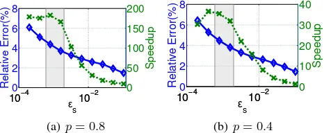
100−4 10−2
Figure 1: Illustration of the relative error and speedup across sample sizes,ǫs. Two levels of sparsity,p, are shown.
The trade-off between relative error and speed.The fun-damental trade-off in the design of the accelerator is between the sample size, ǫs, and the quality of the solution. The
speedup of the framework comes from choosingǫs small,
but if it is chosen too small then the quality of the solution suffers. For the algorithm to provide improvements in prac-tice, it is important for there to be a sweet spot whereǫsis
small and the quality of the solution is still good, as indicated in the shaded region of Figure 1.
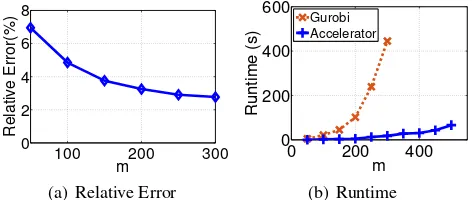
Scalability.In addition to speeding up LP solvers, our ac-celeration framework provides significantly improved scal-ability. Because the LP solver only needs to be run on a (small) sample LP, rather than the full LP, the accelerator provides order of magnitude increase in the size of prob-lems that can be solved. This is illustrated in Figure 2. The figure shows the runtime and relative error of the accel-erator. In these experiments we have fixed p = 0.8 and n/m= 103as we scalem. We have setǫ
s= 0.01
through-out. As (a) shows, one can chooseǫsmore aggressively in
large problems since leavingǫsfixed leads to improved
ac-curacy for large scale problems. Doing this would lead to larger speedups; thus by keepingǫsfixed we provide a
con-servative estimate of the improved scalability provided by the accelerator. The results in (b) illustrate the improvements in scalability provided by the accelerator. Gurobi’s run time grows quickly until finally, it runs into memory errors and cannot arrive at a solution. In contrast, the runtime of the ac-celerator grows slowly and can (approximately) solve prob-lems of much larger size. To emphasize the improvement in scalability, we run an experiment on a laptop with In-tel Core i5 CPU and 8 GB RAM. For a problem with size m = 102, n= 107, Gurobi fails due to memory limits. In contrast, the accelerator produces a solution in 10minutes with relative error less than4%.
The benefits of cloning.Speculative execution is an impor-tant tool that parallel analytics frameworks use to combat the impact of stragglers. Our acceleration framework can imple-ment speculative execution seamlessly by running multiple clones (samples) in parallel and choosing the ones that fin-ish the quickest. We illustrate the benefits associated with cloning in Figure 3. This figure shows the percentage gain in relative error and speedup associated with using different numbers of clones. In these experiments, we fixǫ = 0.002
100 200 300 0
2 4 6 8
m
Relative Error(%)
(a) Relative Error
0 200 400
0 200 400 600
m
Runtime (s)
Gurobi Accelerator
(b) Runtime
Figure 2:Illustration of the relative error and runtime as the problem size,m, grows.
0 20 40
0 5 10 15
Number of Clones
Relative Error Gain(%)
(a) Relative Error
0 20 40
20 40 60 80
Number of Clones
Speedup
(b) Speedup
Figure 3: Illustration of the impact of cloning on solution quality as the number of clones grows.
have finished. Note that the first four clones do not impact the speedup as long as they can be run in parallel. However, for larger numbers of clones our experiments provide a con-servative estimate of the value of cloning since our server only has 8 cores. The improvements would be larger than shown in Figure 3 in a system with more parallelism. De-spite this conservative comparison, the improvements illus-trated in Figure 3 are dramatic. Cloning reduces the rela-tive error of the solution by12%and triples the speedup. Note that these improvements are significant even though the solver we are accelerating is not a parallel solver.
3.3
Case Study
To illustrate the performance in a specific practical setting, we consider an example focused on optimal resource allo-cation in a network. We consider an LP that represents a multi-constraint knapsack problem associated with placing resources at intersections in a city transportation network. For example, we can place public restrooms, advertisements, or emergency supplies at intersections in order to maximize social welfare, but such that there never is a particularly high concentration of resources in any area.
Specifically, we consider a subset of the California road network dataset (Leskovec and Krevl 2014), consisting of
100,000connected traffic intersections. We consider only a subset of a total of1,965,206intersections because Gurobi is unable to handle such a large dataset when run on a laptop with Intel Core i5 CPU and 8 GB RAM. We choose1000of the100,000intersections uniformly at random and defined for each of them a local vicinity of20,000neighboring
inter-0 0.05 0.1
0 5 10 15
ǫs
Relative Error (%)
(a) Relative Error
0 0.05 0.1
0 50 100 150
ǫs
Runtime (s)
Gurobi Accelator
(b) Runtime
Figure 4:Illustration of the relative error and runtime across sample sizes,ǫs, for the real data experiment on the
Califor-nia road network dataset.
sections, allowing overlap between the vicinities. The goal is to place resources strategically at intersections, such that the allocation is not too dense within each local vicinity. Each intersection is associated with a binary variable which repre-sents a yes or no decision to place resources there. Resources are constrained such that the sum of the number of resource units placed in each local vicinity does not exceed10,000.
Thus, the dataset is as follows. Each elementAij in the
data matrix is a binary value representing whether or not the i-th intersection is part of thej-th local vicinity. There are
1000local vicinities and100,000intersections, henceAis a(1000×100,000)matrix. Within each local vicinity, there are no more thanbj = 10,000resource units.
The placement of resources at particular locations has an associated utility, which is a quantifier of how beneficial it is to place resources at various locations. For example, the benefit of placing public restrooms, advertisements, or emer-gency supplies at certain locations may be proportional to the population of the surrounding area. In this problem, we randomly draw the utilities from Unif[1,10]. The objective value is the sum of the utilities at whose associated nodes resources are placed.
Figure 4 demonstrates the relative error and runtime of the accelerator compared to Gurobi, as we vary the sample size ǫs. There is a speed up by a factor of more than30when the
approximation ratio is0.9, or a speed up by a factor of about
9when the approximation ratio is0.95.
4
Proofs
In this section we present the technical lemmas used to prove Theorem 3.1. The approach of the proof is inspired by the techniques in (Agrawal, Wang, and Ye 2014); how-ever the analysis in our case is more involved. This is due to the fact that our result applies to approximate LP solvers while the techniques in (Agrawal, Wang, and Ye 2014) only apply to exact solvers. For example, this leads our framework to have three error parameters (ǫs, ǫf, αd)
while (Agrawal, Wang, and Ye 2014) has a single error pa-rameter.
(Lemma 4.7). In both cases, we use the following concen-tration bound, e.g., (van der Vaart and Wellner 1996). Theorem 4.1 (Hoeffding-Bernstein Inequality). Let u1, u2. . . , usbe random samples without replacement from
Step 1: The solution is feasible
Lemma 4.2. LetAbe a(αp, αd)-approximation algorithm
for packing LPs, αp, αd ≥ 1. For any ǫs > 0, ǫf ≥ q
6(m+2) logn
ǫsB , the solution Algorithm 1 gives to LP(1) is
feasible with probability at least1−1/2n, where the prob-ability is over the choice of samples.
Proof. Define aprice-realization,R(φ), of a price vectorφ as the set{rij = aijxj(φ), j ∈ [n], i ∈ [m]} (note that
rij ∈ {0, aij}) and denote, a “row” of R(φ)as Ri(φ) =
{rij =aijxj(φ), j ∈ [n]}. We say thatRi(φ)isinfeasible
ifP
j∈[n]rij > bi. The approach of this proof is to bound
the probability that, for a given sample, the sample LP is feasible while there is someifor whichRi(φ)is not feasible
in the original LP.
To begin, note that it naively seems that there are2n
pos-sible realizations ofR(φ), over all possible price vectorsφ, asxj ∈ {0,1}. However, a classical result of combinatorial
geometry (Orlik and Terao 1992) shows that there are only nm
possible realizations since eachR(φ)is characterized by a separation ofnpoints({cj, aj}nj=1)in anm-dimensional plane by a hyperplane, whereajdenotes thej-th column of
A. The maximal number of such hyperplanes isnm.
Next, we define a sampleS ⊂[n],|S|=ǫsnasRi-good
claim relates these two definitions.
Claim 4.3. If a sampleSisx˜i-good thenSisRi-good.
Proof. Denote the dual solution of the sample LP byy˜ = [ ˜φ,ψ˜]. The dual complementary slackness conditions im-ply that, if ψ˜j > 0 then α1
which shows thatSisRi-good, completing the proof.
Next, fix the LP andR(φ). For the purpose of the proof, choosei ∈ [n]uniformly at random. Next, we sampleǫsn
elements without replacement fromnvariables taking the
values{rij}. Call this sampleS. LetX =Pj∈Srij be the
random variable denoting the sum of these random variables. Note that E[X] = ǫsPj∈Nrij, where the expectation is
over the choice ofS, and that the eventsP
j∈Nrij > biand
To complete the proof, we now take a union bound over all possible realizations ofR, which we bounded earlier by nm
, and values ofi.
Step 2: The solution is close to optimal
To prove that the solution is close to optimal we make two mild, technical assumptions.
Assumption 4.4. For any dual pricesy = [φ, ψ], there are at mostmcolumns such thatφTa
j =cj.
Assumption 4.5. AlgorithmAmaintains primal and dual solutionsxandy = [φ, ψ]respectively withψ >0only if Pn
j=1aijxj< cj.
Assumption 4.4 does not always hold; however it can be enforced by perturbing each cj by a small
amount at random (see, e.g., (Devanur and Hayes 2009; Agrawal, Wang, and Ye 2014)). Assumption 4.5 holds for any “reasonable”(1−αd)-approximation dual ascent
algo-rithm, and any algorithm that does not satisfy it can easily be modified to do so. These assumptions are used only to prove the following claim, which is used in the proof of the lemma that follows.
inition of the allocation rule (recall that if ψ˜j > 0 then P
difference between them must occur forjsuch thatψ˜j = 0. hold that˜xj= 0by complementary slackness, but then also
xj( ˜φ) = 0by the allocation rule. Assumption 4.4 then
com-probability at least1−21n, where the probability is over the
choice of samples.
Proof. Denote the primal and dual solutions to the sampled LP in (2) of Algorithm 1 byx,˜ y˜= [ ˜φ,ψ˜]. For purposes of the proof, we construct the following related LP.
maximize Pn
Note that ˜b has been set to guarantee that the LP is al-ways feasible, and thatx( ˜φ)andy∗ = [ ˜φ, ψ∗]
satisfy the (exact) complementary slackness conditions, whereψ∗
j =
cj −P m
i=1aij ifxj( ˜φ) = 1, andψj∗ = 0ifxj( ˜φ)6= 1. In
particular, note thatψ∗ preserves the exact complementary
slackness condition, asψ∗
j is set to zero whenxj( ˜φ) 6= 1.
Thereforex( ˜φ) andy∗ = [ ˜φ, ψ∗]are optimal solutions to
LP (6).
A consequence of the approximate dual complementary slackness condition for the solutionx,˜ y˜is that thei-th pri-mal constraint of LP (2) is almost tight whenφ˜i>0:
This allows us to boundP
j∈Saijxj( ˜φ)as follows.
where the first inequality follows from Claim 4.6 and the second follows from the fact thatB ≥m(αd)2
adjusted if application for largerαdis desired.
Applying the union bound gives that, with probability at least1− 1
is a feasible solution to LP (6). Thus, the optimal value of LP (6) is at least (1−3ǫf)
(αd)2
Pn j=1cjx∗j.
References
[Agrawal, Klein, and Ravi 1995] Agrawal, A.; Klein, P.; and Ravi, R. 1995. When trees collide: An approximation algo-rithm for the generalized steiner problem on networks.SIAM J. on Comp.24(3):440–456.
[Agrawal, Wang, and Ye 2014] Agrawal, S.; Wang, Z.; and Ye, Y. 2014. A dynamic near-optimal algorithm for online linear programming. Oper. Res.62(4):876–890.
[Allen-Zhu and Orecchia 2015] Allen-Zhu, Z., and Orec-chia, L. 2015. Using optimization to break the epsilon barrier: A faster and simpler width-independent algorithm for solving positive linear programs in parallel. InProc. of SODA, 1439–1456.
[Ananthanarayanan et al. 2010] Ananthanarayanan, G.; Kandula, S.; Greenberg, A. G.; Stoica, I.; Lu, Y.; Saha, B.; and Harris, E. 2010. Reining in the outliers in map-reduce clusters using mantri. InProc. of OSDI.
[Ananthanarayanan et al. 2013] Ananthanarayanan, G.; Gh-odsi, A.; Shenker, S.; and Stoica, I. 2013. Effective straggler mitigation: Attack of the clones. InProc. of NSDI, 185–198. [Ananthanarayanan et al. 2014] Ananthanarayanan, G.; Hung, M. C.-C.; Ren, X.; Stoica, I.; Wierman, A.; and Yu, M. 2014. Grass: Trimming stragglers in approximation analytics. InProc. of NSDI, 289–302.
[Awerbuch and Khandekar 2008] Awerbuch, B., and Khan-dekar, R. 2008. Stateless distributed gradient descent for positive linear programs. InProc. of STOC, STOC ’08, 691. [Balakrishnan, Magnanti, and Wong 1989] Balakrishnan,
A.; Magnanti, T. L.; and Wong, R. T. 1989. A dual-ascent procedure for large-scale uncapacitated network design. Oper. Res.37(5):716–740.
[Bar-Yehuda and Even 1981] Bar-Yehuda, R., and Even, S. 1981. A linear-time approximation algorithm for the weighted vertex cover problem. J. of Algs.2(2):198 – 203. [Bartal, Byers, and Raz 2004] Bartal, Y.; Byers, J. W.; and
Raz, D. 2004. Fast distributed approximation algorithms for positive linear programming with applications to flow control. SIAM J. on Comp.33(6):1261–1279.
[Bertsimas and Vohra 1998] Bertsimas, D., and Vohra, R. 1998. Rounding algorithms for covering problems. Math. Prog.80(1):63–89.
[Boyd and Vandenberghe 2004] Boyd, S., and Vanden-berghe, L. 2004. Convex Optimization. Cambridge University Press.
[Buchbinder and Naor 2009] Buchbinder, N., and Naor, J. 2009. The design of competitive online algorithms via a primal-dual approach. Found. and Trends in Theoretical Computer Science3(2-3):93–263.
[Burger et al. 2012] Burger, M.; Notarstefano, G.; Bullo, F.; and Allgower, F. 2012. A distributed simplex algorithm for degenerate linear programs and multi-agent assignment. Automatica48(9):2298–2304.
[Byers and Nasser 2000] Byers, J., and Nasser, G. 2000. Utility-based decision-making in wireless sensor networks. InMobile and Ad Hoc Networking and Comp., 143–144. [Candes and Plan 2011] Candes, E., and Plan, Y. 2011. Tight
oracle inequalities for low-rank matrix recovery from a min-imal number of noisy random measurements. IEEE Trans. on Info. Theory57(4):2342–2359.
[Candes, Romberg, and Tao 2006] Candes, E.; Romberg, J.; and Tao, T. 2006. Robust uncertainty principles: Exact sig-nal reconstruction from highly incomplete frequency infor-mation. IEEE Trans. Inform. Theory52(2):489 – 509. [Devanur and Hayes 2009] Devanur, N. R., and Hayes, T. P.
2009. The adwords problem: online keyword matching with budgeted bidders under random permutations. InProc. of EC, 71–78.
[Donoho and Tanner 2005] Donoho, D. L., and Tanner, J. 2005. Sparse nonnegative solution of underdetermined lin-ear equations by linlin-ear programming. InProc. of the Na-tional Academy of Sciences of the USA, 9446–9451. [Donoho 2006] Donoho, D. L. 2006. Compressed sensing.
IEEE Trans. Inform. Theory52:1289–1306.
[Erlenkotter 1978] Erlenkotter, D. 1978. A dual-based procedure for uncapacitated facility location. Oper. Res. 26(6):992–1009.
[Goemans and Williamson 1995] Goemans, M. X., and Williamson, D. P. 1995. A general approximation tech-nique for constrained forest problems. SIAM J. on Comp. 24(2):296–317.
[Leskovec and Krevl 2014] Leskovec, J., and Krevl, A. 2014. SNAP Datasets: Stanford large network dataset col-lection.http://snap.stanford.edu/data. [London et al. 2017] London, P.; Chen, N.; Vardi, S.; and
Wierman, A. 2017. Distributed optimization via local computation algorithms. http://users.cms.caltech.edu/ plon-don/loco.pdf.
[Luby and Nisan 1993] Luby, M., and Nisan, N. 1993. A parallel approximation algorithm for positive linear pro-gramming. InProc. of STOC, 448–457.
[Mansour et al. 2012] Mansour, Y.; Rubinstein, A.; Vardi, S.; and Xie, N. 2012. Converting online algorithms to local computation algorithms. InProc. of ICALP, 653–664. [Mohan et al. 2014] Mohan, K.; London, P.; Fazel, M.;
Wit-ten, D.; and Lee, S.-I. 2014. Node-based learning of multiple gaussian graphical models.JMLR15:445–488.
[Nesterov 2005] Nesterov, Y. 2005. Smooth minimization of non-smooth functions.Math. Prog.103(1):127–152. [Notarstefano and Bullo 2011] Notarstefano, G., and Bullo,
F. 2011. Distributed abstract optimization via constraints consensus: Theory and applications. IEEE Trans. Autom. Control56(10):2247–2261.
[Orlik and Terao 1992] Orlik, P., and Terao, H. 1992. Ar-rangements of Hyperplanes. Grundlehren der mathematis-chen Wissenschaften. Springer-Verlag Berlin Heidelberg. [Plotkin, Shmoys, and Tardos 1995] Plotkin, S. A.; Shmoys,
D. B.; and Tardos, E. 1995. Fast approximation algo-rithms for fractional packing and covering problems. Math. of Oper. Res.20(2):257–301.
[Ravikumar, Agarwal, and Wainwright 2010] Ravikumar, P.; Agarwal, A.; and Wainwright, M. J. 2010. Message passing for graph-structured linear programs: Proximal methods and rounding schemes. JMLR11:1043–1080.
[Recht, Fazel, and Parrilo 2010] Recht, B.; Fazel, M.; and Parrilo, P. A. 2010. Guaranteed minimum-rank solutions of linear matrix equations via nuclear norm minimization. SIAM Review52(3):471–501.
[Ren et al. 2015] Ren, X.; Ananthanarayanan, G.; Wierman, A.; and Yu, M. 2015. Hopper: Decentralized speculation-aware cluster scheduling at scale. InProc. of SIGCOMM. [Richert and Cort´es 2015] Richert, D., and Cort´es, J. 2015.
Robust distributed linear programming.Trans. Autom. Con-trol60(10):2567–2582.
[Riquelme, Johari, and Zhang 2017] Riquelme, C.; Johari, R.; and Zhang, B. 2017. Online active linear regression via thresholding. InProc. of AAAI.
[Sanghavi, Malioutov, and Willsky 2008] Sanghavi, S.; Malioutov, D.; and Willsky, A. S. 2008. Linear program-ming analysis of loopy belief propagation for weighted matching. InProc. of NIPS, 1273–1280.
[Sridhar et al. 2013] Sridhar, S.; Wright, S. J.; R´e, C.; Liu, J.; Bittorf, V.; and Zhang, C. 2013. An approximate, efficient LP solver for LP rounding. InProc. of NIPS, 2895–2903. [Taskar, Chatalbashev, and Koller 2004] Taskar, B.;
Chatal-bashev, V.; and Koller, D. 2004. Learning associative markov networks. InProc. of ICML.
[Trevisan 1998] Trevisan, L. 1998. Parallel approximation algorithms by positive linear programming. Algorithmica 21(1):72–88.
[van der Vaart and Wellner 1996] van der Vaart, A., and Wellner, J. 1996. Weak Convergence and Empirical Pro-cesses With Applications to Statistics. Springer Series in Statistics. Springer-Verlag New York.
[Woodruff 2014] Woodruff, D. P. 2014. Sketching as a tool for numerical linear algebra.Found. and Trends in Theoret-ical Computer Science10(1-2):1–157.
[Young 2001] Young, N. E. 2001. Sequential and parallel al-gorithms for mixed packing and covering. InProc. of FOCS, 538–546.
[Yuan and Lin 2007a] Yuan, M., and Lin, Y. 2007a. Model selection and estimation in the gaussian graphical model. Biometrika94(10):19–35.